Performs between group PCA allowing for leave-one-out cross-validation, which is useful one the number of variables exceeds the number of observations (i.e., alleviates spurious separation between groups).
bg_prcomp(
  x,
  groups,
  gweights = TRUE,
  LOOCV = FALSE,
  recompute = FALSE,
  corr = FALSE
)
Arguments
- x
A matrix with variables as columns and observations as rows.
- groups
Factor; classification of observations of
xinto a priori groups.- gweights
Logical; whether to weight each group by its number of observations.
- LOOCV
Logical; whether to apply leave-one-out cross-validation.
- recompute
Logical; whether to re-compute rotation matrix using the scores resulting from LOOCV.
- corr
Logical; whether to use correlation instead of covariance matrix as input.
Value
A "bg_prcomp" object formatted following the "prcomp"
class:
$x:a matrix with the scores of observations in the new ordination axes.$sdev:the standard deviations of the principal components (i.e., the square roots of the singular values of the covariance or correlation matrix).$rotation:an x (g - 1)matrix of eigenvector coefficients (withgbeing the number of groups.$center:the mean values of the original variables for the entire sample (i.e., the grand mean).$grcenters:the mean values of the original variables for each group.$totvar:the sum of the variances of the original data.
Details
bgPCA finds the liner combination of variables (which in the
context of morphospace will generally be a series of shapes
arranged as 2-margin matrix) maximizing variation between groups'
centroids, and then project the actual observation into the resulting
ordination axes. This method is preferred here to LDA/CVA as a way to
produce ordinations maximizing separation between groups because it avoids
spherization of shape variation carried out for the former methods.
Recently, it has been pointed out that bgPCA produces spurious separation between groups when the number of variables exceeds the number of observations (which is a common situation in geometric morphometrics analyses). This problem can be alleviated by carrying out a leave-one-out cross-validation (LOOCV; i.e., each observation is excluded from the calculation of bgPCA prior to its projection in the resulting ordination as a way to calculate its score).
The dimensionality of the ordination space generated by bgPCA will be equal to the number of groups minus one, the number of original variables, or the number of observations, whichever is lower.
References
Mitteroecker, P., & Bookstein, F. (2011). Linear discrimination, ordination, and the visualization of selection gradients in modern morphometrics. Evolutionary Biology, 38(1), 100-114.
Bookstein, F. L. (2019). Pathologies of between-groups principal components analysis in geometric morphometrics. Evolutionary Biology, 46(4), 271-302.
Cardini, A., O'Higgins, P., & Rohlf, F. J. (2019). Seeing distinct groups where there are none: spurious patterns from between-group PCA. Evolutionary Biology, 46(4), 303-316.
Cardini, A., & Polly, P. D. (2020). Cross-validated between group PCA scatterplots: A solution to spurious group separation?. Evolutionary Biology, 47(1), 85-95.
Rohlf, F. J. (2021). Why clusters and other patterns can seem to be found in analyses of high-dimensional data. Evolutionary Biology, 48(1), 1-16.
Thioulouse, J., Renaud, S., Dufour, A. B., & Dray, S. (2021). Overcoming the spurious groups problem in between-group PCA. Evolutionary Biology, 48(4), 458-471.
Examples
#load data
library(magrittr)
data("shells")

#extract species classification and shapes
species <- shells$data$species
shapes <- shells$shapes$coe

#perform between-groups PCA
bgpca <- bg_prcomp(x = shapes, groups = species)

#inspect results
names(bgpca) #the contents of the resulting object
#> [1] "sdev"      "rotation"  "x"         "center"    "grcenters" "totvar"
exp_var(bgpca) #variance explained by each axis
#>         variance cummulative
#> bgPC1  115.74130    115.7413
#> bgPC2    4.54123    120.2825
#> bgPC3    0.34279    120.6253
#> bgPC4         NA          NA
#> bgPC5         NA          NA
#> bgPC6         NA          NA
#> bgPC7         NA          NA
#> bgPC8         NA          NA
#> bgPC9         NA          NA
#> bgPC10        NA          NA
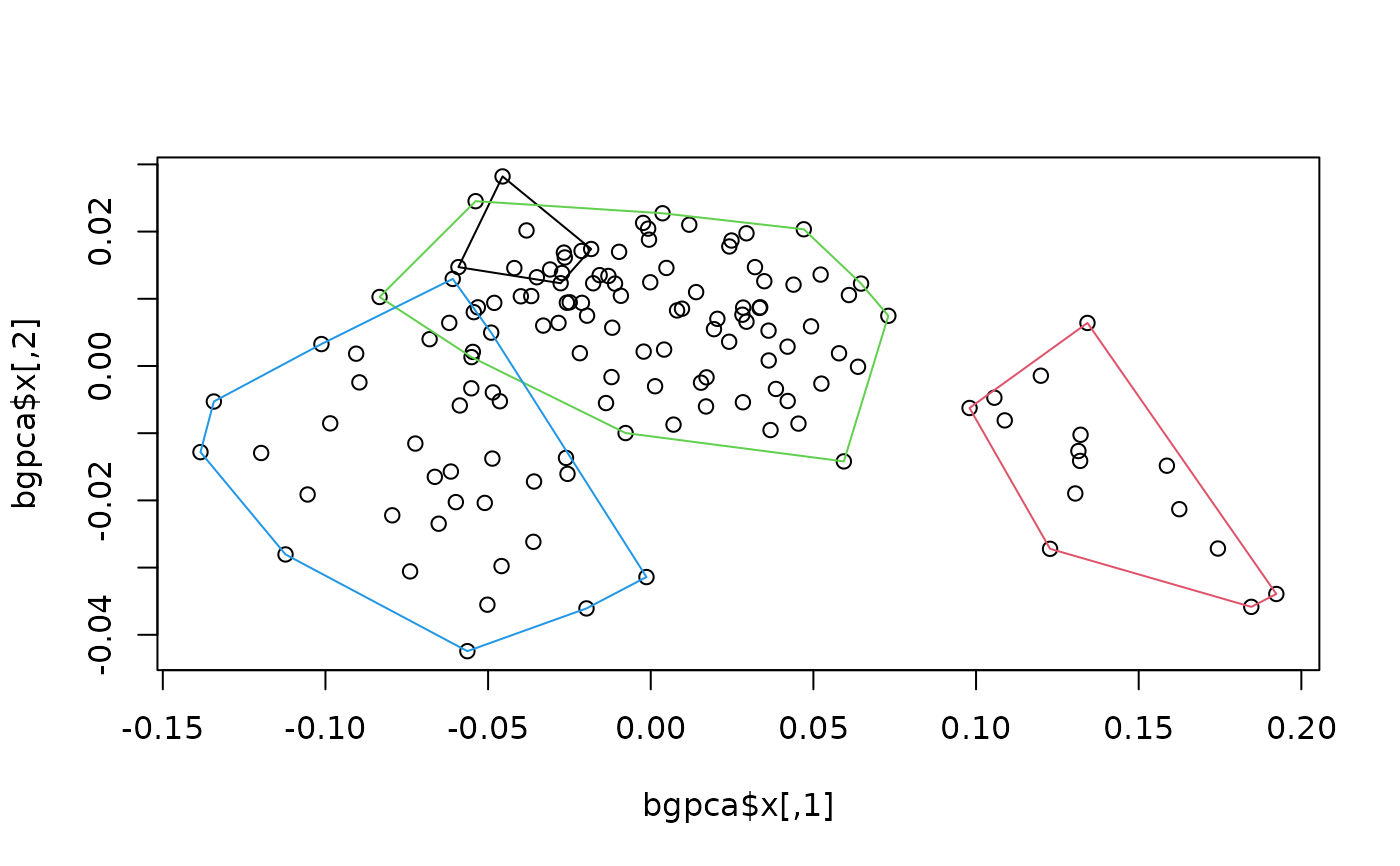
plot(bgpca$x) #ordination
hulls_by_group_2D(bgpca$x, species) #add convex hulls for species


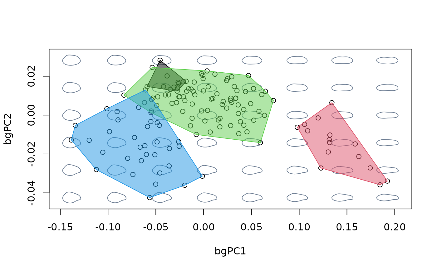
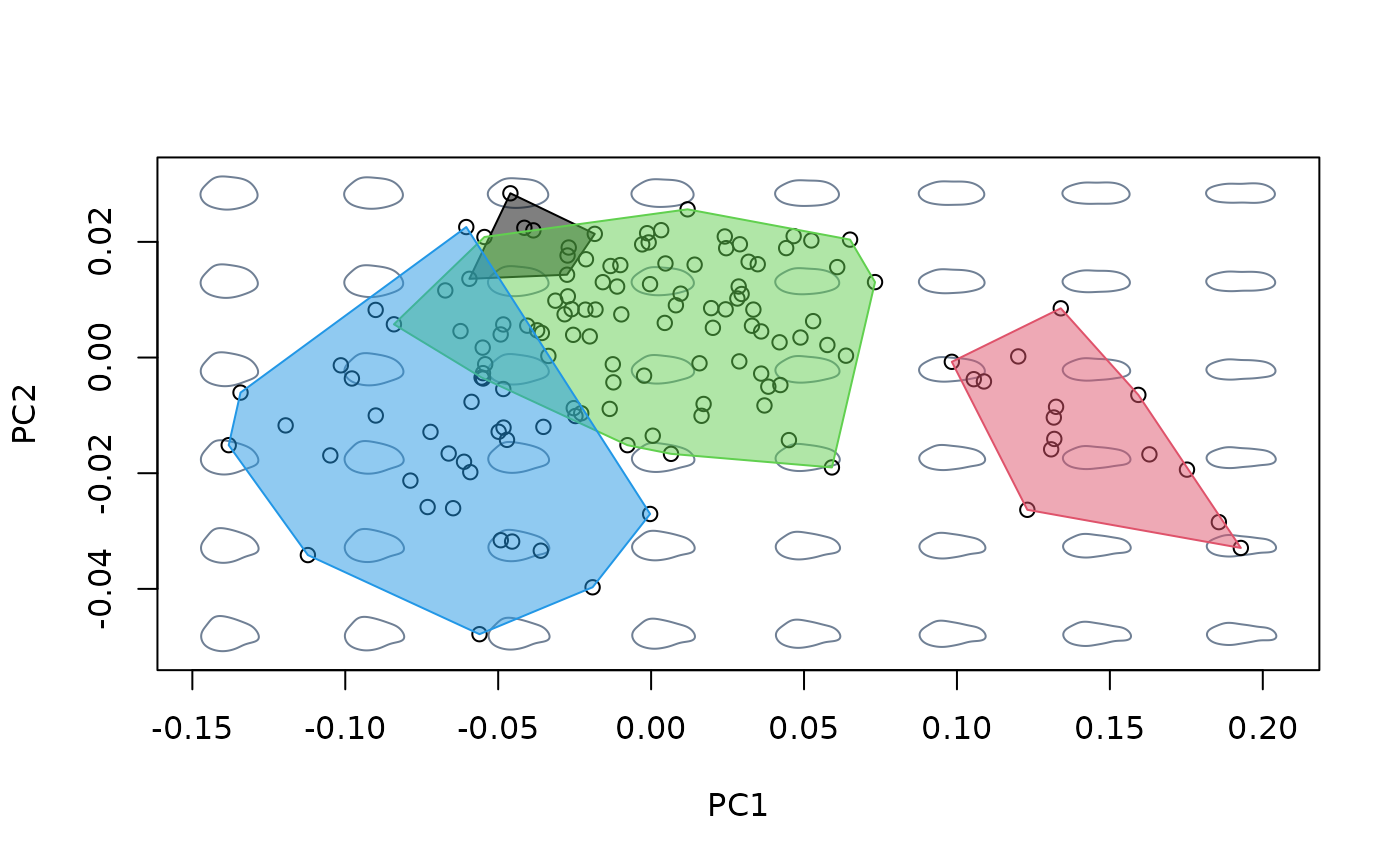
#compare shape variation as summarized by different methods

#build morphospace using between-groups PCA
mspace(shapes, links = links, nh = 8, nv = 6, FUN = bg_prcomp,
       groups = species) %>%
  proj_shapes(shapes) %>%
  proj_groups(shapes, groups = species, alpha = 0.5)


#compare against morphospace built with ordinary PCA
mspace(shapes, links = links, nh = 8, nv = 6, invax = c(1,2)) %>%
  proj_shapes(shapes) %>%
  proj_groups(shapes, groups = species, alpha = 0.5)
