Worked examples

morphospace has been built to handle the most common types of geometric morphometrics data that can be found in the paleobiological and evolutionary biology literature. Below, the general capabilities of this package are showcased using three data sets representing these data types and various spatio-temporal scales that are typically addressed when studying evolutionary variation.

2D Landmark data

Most of the capabilities for 2D landmark data visualization has been already covered in General usage. This section will quickly show how to use a curve or set of curves outlining aspects of the phenotype not captured by the chosen landmarks to improve visualizations via TPS interpolation. To do so we use the wings data set, which has been taken from Soto et al. (2012) and includes wing shape data from 263 experimentally bred specimens belonging to two recently diverged cactophilic Drosophila species, D. koepferae and D. buzzattii. These two species show preference to different host cacti (columnar cacti from the genus Trichocereus and prickly pears from the genus Opuntia, respectively) and are considered morphologically cryptic (usually, they can be recognized only from genital morphology). The data set include the centroid size of each wing, as well as information on the host cacti each specimen was bred on, its species, sex, isofemale line, and replica. Also included is a template containing a series of curves describing wing outline and veins (created using build_template2d), which will be warped using TPS interpolation and used to generate fancy shape models for our morphospace.

# Load morphospace as well as geomorph and magrittr
library(morphospace)
library(geomorph)
library(magrittr)

# Load wing data and extract shapes, centroid sizes, classification 
# of sex and species, links between landmarks, template, and phylogeny
data("wings")

shapes <- wings$shapes
sizes <- log(wings$sizes)
species <- wings$data$species
cactus <- wings$data$cactus
line <- wings$data$line
sex <- wings$data$sex
replica <- wings$data$replica
curvs <- wings$template


# Inspect shapes using links
pile_shapes(shapes, wings$links)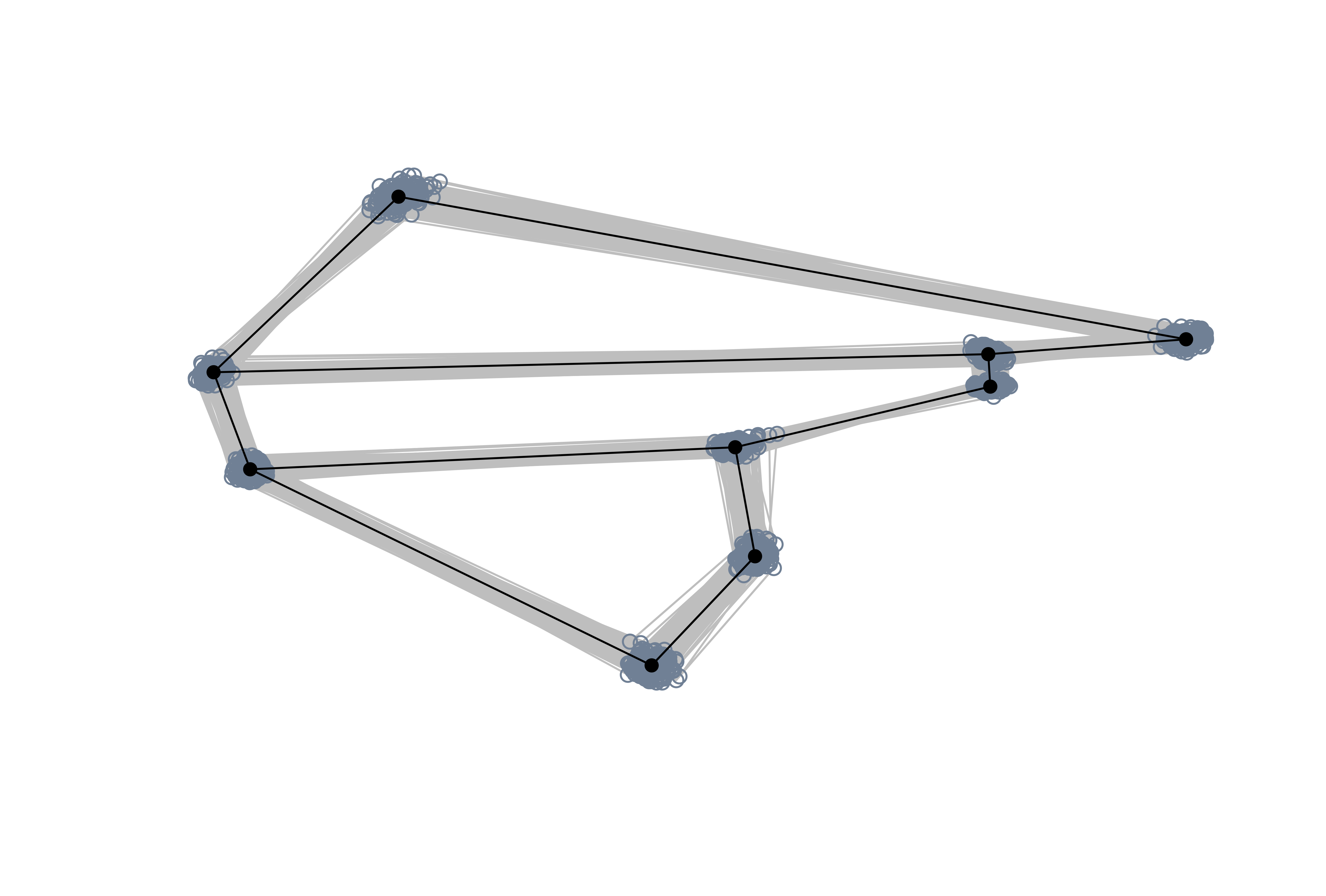

# Generate morphospace but use warped wings as background models
spxcac <- species:cactus
mspace(shapes, template = curvs, col.ldm = "black", cex.ldm = 5, plot = FALSE) %>%
  proj_shapes(shapes = shapes, 
              col = rep(c("blue", "orange"), each = 2)[spxcac], 
              pch = rep(c(16, 1), times = 2)[spxcac]) %>%
  proj_groups(shapes = shapes, groups = spxcac, ellipse = TRUE, 
              col = rep(c("blue", "orange"), each = 2), 
              lty = rep(c(1, 2), times = 2), lwd = 2) %>%
  plot_mspace(legend = TRUE, cex.legend = 1.5)
title("Morphospace using template")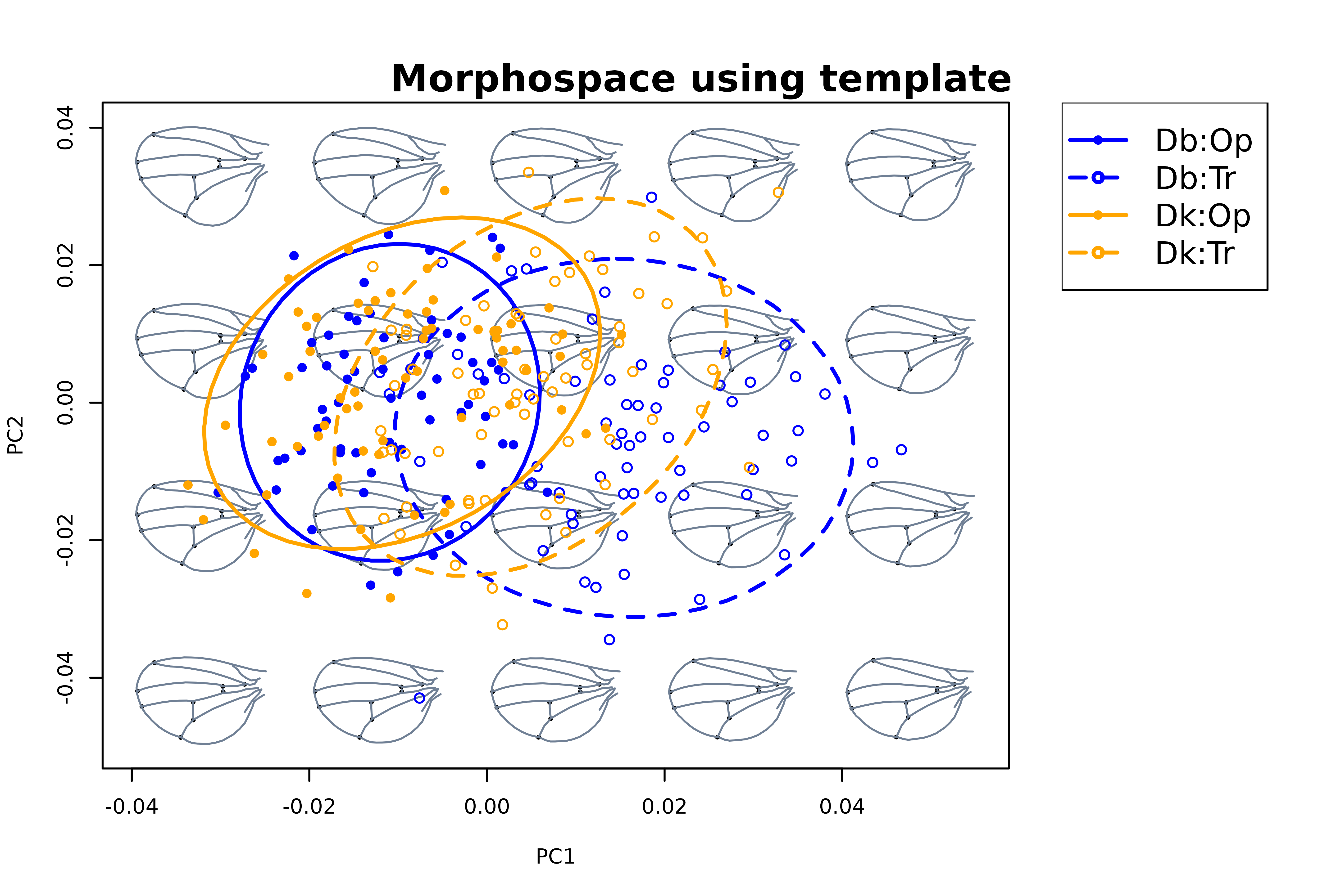

Assume for a second we are interested in exploring whether we can identify morphological differences between species. The pattern we are seeing suggets that variation in wing morphology is very subtle, that wings of these two species are basically indistinguishable, and that cactus has a large effect on wing morphology. However, there is a lot of ‘noise’ (i.e. sexual dimorphism, allometric variation, genetic variation, even host cactus) we can get rid of using detrend_shapes. We do this species-wise, so that patterns of interspecific variation are not blurred.

detr_shapes <- shapes * 0
for(i in 1:2) {
  index <- species == levels(species)[i]
  subshapes <- shapes[,,index]
  subsex <- sex[index]
  subline <- line[index]
  subreplica <- replica[index]
  subsizes <- sizes[index]
  subcactus <- cactus[index]

  subdetr_shapes1 <- lm(two.d.array(subshapes) ~ subsex * subline * subreplica) %>%
    detrend_shapes(method = "residuals") %>% arrayspecs(p = 9, k = 2)

  subdetr_shapes2 <- lm(two.d.array(subdetr_shapes1) ~ subsizes) %>%
    detrend_shapes(xvalue = max(subsizes), method = "residuals") %>% arrayspecs(p = 9, k = 2)

  subdetr_shapes3 <- lm(two.d.array(subdetr_shapes2) ~ subcactus) %>%
    detrend_shapes(xvalue = c("Op", "Tr")[i], method = "residuals") %>% arrayspecs(p = 9, k = 2)

  detr_shapes[,,index] <- subdetr_shapes3
}

(Note: we do this in several step for a good reason: when we use detrend_shapes to detrend shape variation, the grand mean is used by default as the new mean shape of the sample; however by specifying a value or level of x from the model in the xvalue argument, we can use that new value as the mean shape for our ‘detrended’ shape variation. In this case, we are analitically displacing all the wings to the shapes they should have if reared in their primary host cactus, and attained their species’ maximum size).

Once shape variation has been ‘refined’, we can ordinate it again, and magnify variation so the representation can be more easily interpreted using the mag argument.

mspace(detr_shapes, template = curvs, col.ldm = "black",
       cex.ldm = 5, mag = 2, plot = FALSE) %>%
  proj_shapes(shapes = detr_shapes, 
              col = rep(c("blue", "orange"), each = 2)[spxcac], 
              pch = rep(c(16, 1), times = 2)[spxcac]) %>%
  proj_groups(groups = spxcac, ellipse = TRUE, 
              col = rep(c("blue", "orange"), each = 2), 
              lty = rep(c(1, 2), times = 2), lwd = 2) %>% 
  plot_mspace(legend = TRUE, cex.legend = 1.5)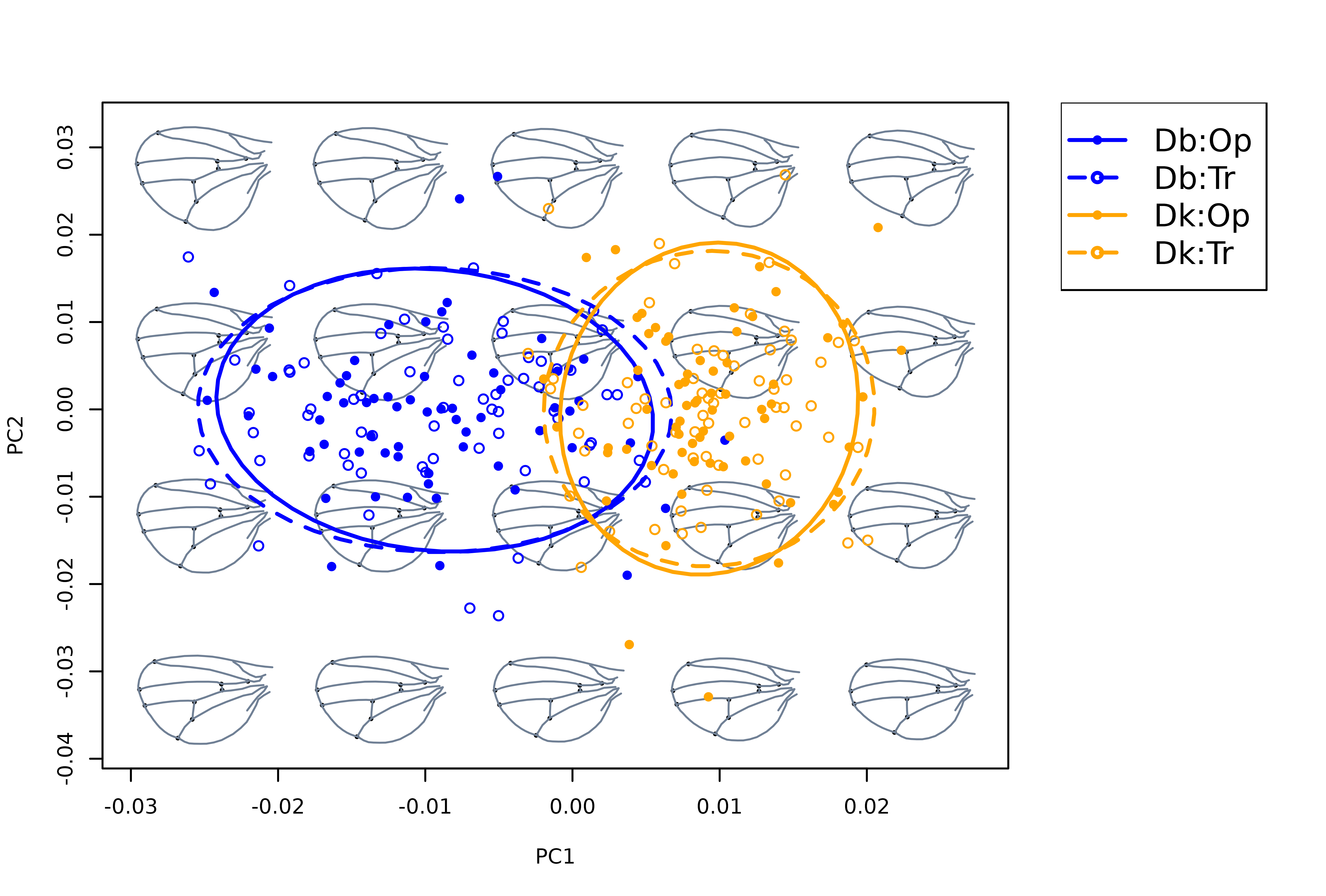

So, after ‘cleaning’ the raw variation interspecific differences become apparent with each species occupying different regions of wing morphospace (elongated and more triangular in D. koepferae, relatively higher and more rounded in D. buzzattii).

Closed outlines

morphospace can also handle closed outline data in the form of Fourier coefficients resulting from an elliptic Fourier analysis. For the purposes of import, normalize and and analize this data we rely on the Momocs package, and use its "OutCoe" format for storing closed outlines as starting point. Below the mspace %>% proj_* workflow is applied to the shells data set taken from Milla Carmona et al. (2018). This include data from 137 specimens belonging to 4 species of the extinct bivalve genus Ptychomya, tracking their shape changes through a 5 million years interval from the Lower Cretaceous of Argentina. The data set includes the information about the shape (measured using 7 harmonics), centroid size, geochronologic age (both relative and absolute), geographic provenance, and taxonomic classification of each specimen.

#Load packages
library(Momocs)
library(magrittr)
library(morphospace)


# Load data from shells, extract shapes, sizes and classification into
# species, absolute and relative ages
data("shells")

shapes <- shells$shapes$coe
sizes <- log(shells$sizes)
species <- shells$data$species
ages <- shells$data$age
bzones <- shells$data$zone


# Pile shapes
pile_shapes(shapes)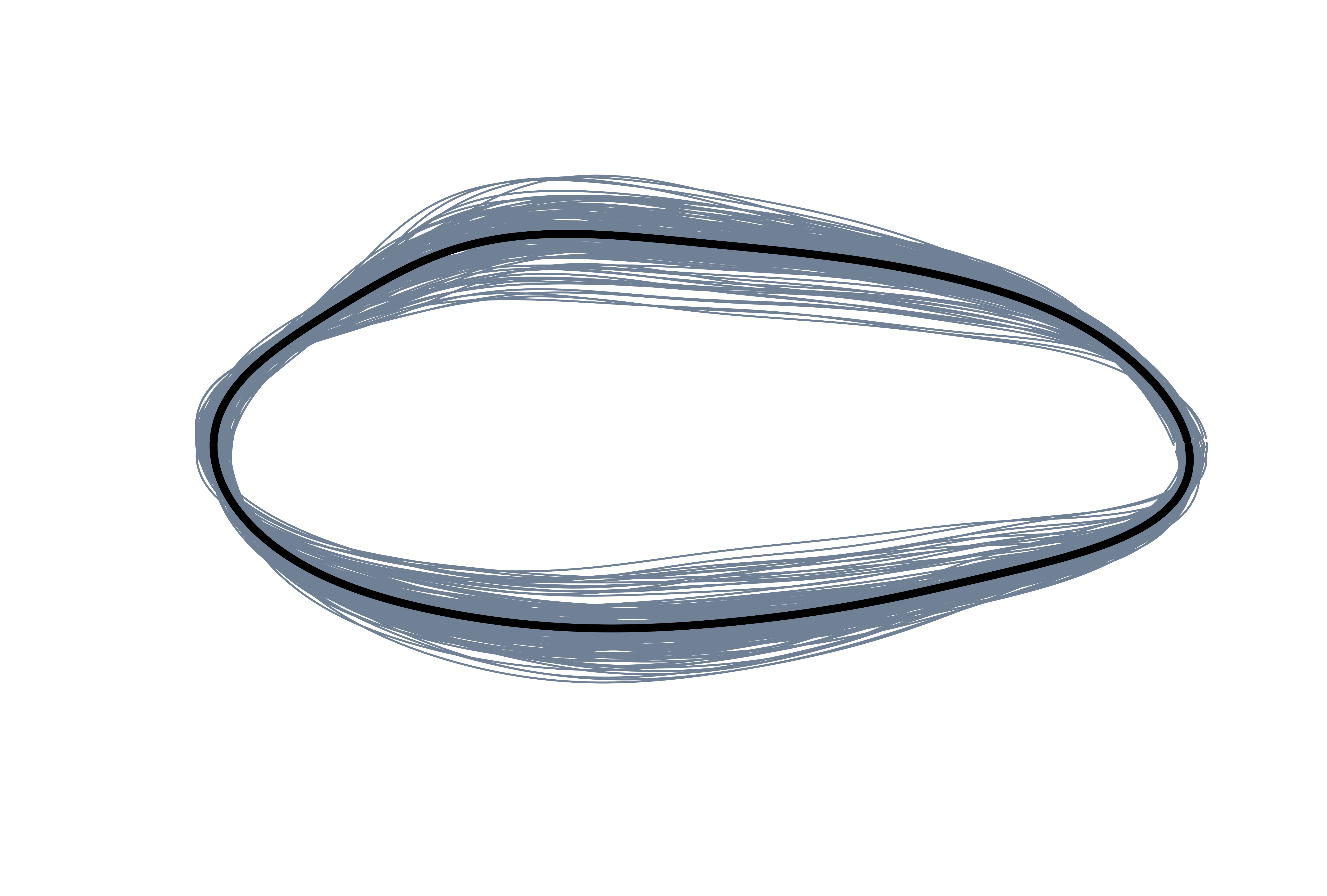

# Generate morphospace using raw variation
mspace(shapes, bg.model = "light gray", plot = FALSE) %>%
  proj_shapes(shapes = shapes, col = species) %>%
  proj_groups(shapes = shapes, groups = species, alpha = 0.5) %>% 
  proj_shapes(shapes = expected_shapes(shapes, species), bg = 1:4, pch = 21) %>% 
  plot_mspace(legend = TRUE, cex.legend = 1)
title("Morphospace")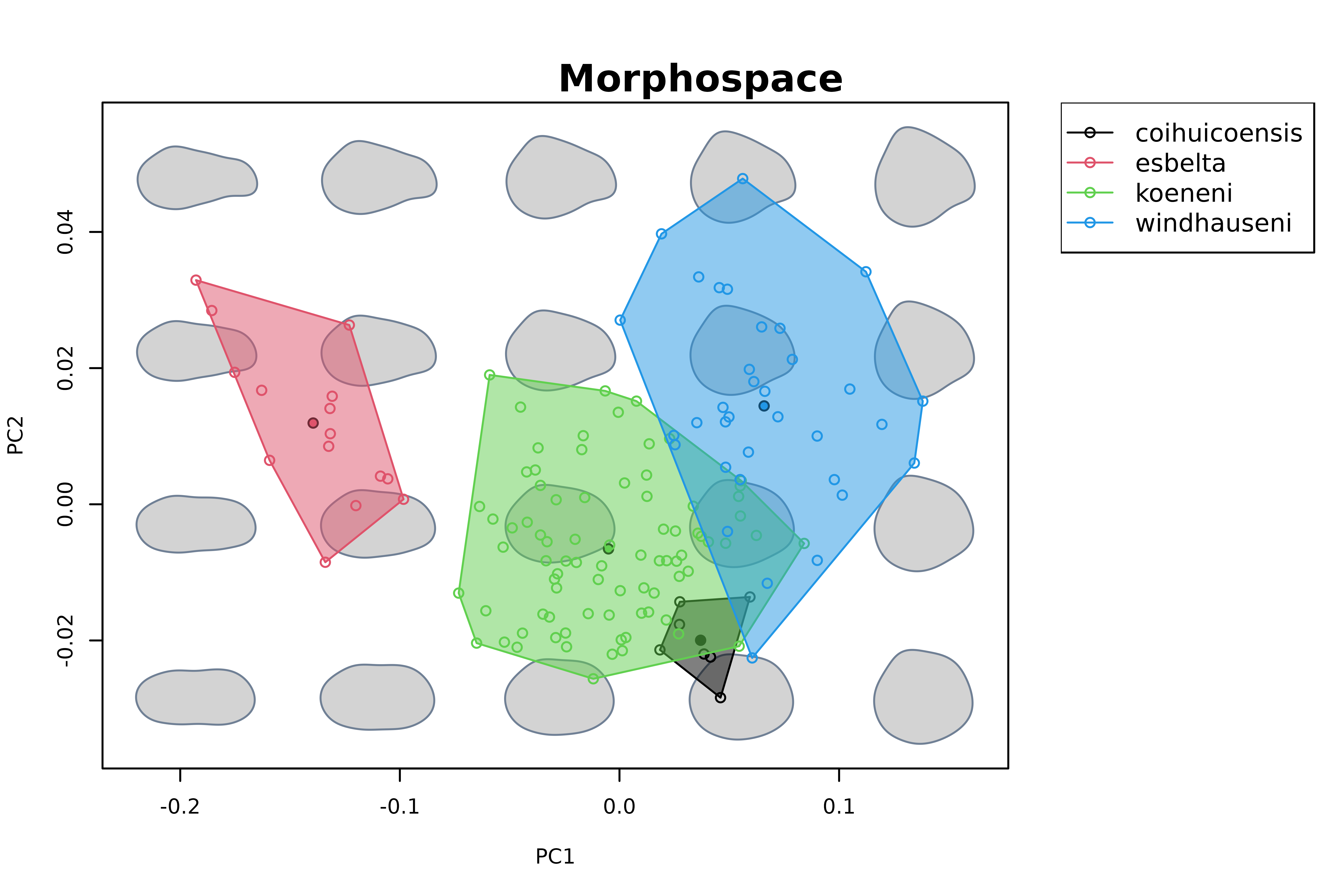

In this case, we are interested in the anagenetic variation shown by each species throughout the studied interval. As before, we can use detrend_shapes to remove variation associated to nuisance factors (in this case, allometric variation). We do this for species separately, and then use expected_shapes to extract their mean shapes.

# 'Clean' shapes separately for each species, removing 1) variation
#associated to geographic provenance and 2) allometric variation
detr_shapes <- shapes * 0
for(i in 1:nlevels(species)) {
  index <- species == levels(species)[i]
  subdetr_shapes <- lm(shapes[index,] ~ sizes[index]) %>% detrend_shapes(xvalue = max(sizes[index]), method = "residuals")
  detr_shapes[rownames(detr_shapes) %in% rownames(subdetr_shapes),] <- subdetr_shapes
}

Note that we don’t need arrayspecs when using detrend_shapes here, that’s because Fourier coefficients are already stored in matrix format).

Now we can use plot_mspace again to create a more complex hybrid plot combining shape changes associated to PC1 against the time axis. To do so, we first do a bit of variable manipulation to obtain 1) a factor combining species classification and relative age (i.e. biozones), and 2) the mean shapes and 3) mean ages of the resulting levels. Then, we build the morphospace (this time, using detrended shapes and between-groups PCA).

(Note: in this case, two separate instances of proj_shapes are used: one for projecting the sampled shapes, and another one to project the mean shape of each species in each biozone. The corresponding scores are stored together in the order in which shapes were projected; see next chunk for an example of how to call them.)

# Combine levels of species and biozones, then compute 1) the mean shapes
# 2) the mean ages of the resulting groups
sp.bz <- factor(species:bzones)
shapes_agesxspecies <- expected_shapes(detr_shapes, sp.bz)
mean_ages <- tapply(ages, sp.bz, mean)

# Generate morphospace (use an additional instance of proj_shapes to project
# the mean shapes of species:biozones)
msp <- mspace(detr_shapes, FUN = bg_prcomp, groups = species,
              mag = 0.5, bg.model = "light gray") %>%
  proj_shapes(shapes = shapes_agesxspecies, pch = 21, 
              bg = c(rep(1,3), rep(2,6), rep(3,9), rep(4,3)), cex = 1.2) %>% 
  proj_shapes(shapes = detr_shapes, col = species) %>%
  proj_groups(shapes = detr_shapes, groups = species, alpha = 0.2)


# Add anagenetic trajectories in morphospace
for(i in 1:4) {
  index <- grepl(x = rownames(msp$projected$scores), pattern = levels(species)[i])
  points(msp$projected$scores[index,], type = "l", lwd = 2, col = i)
}

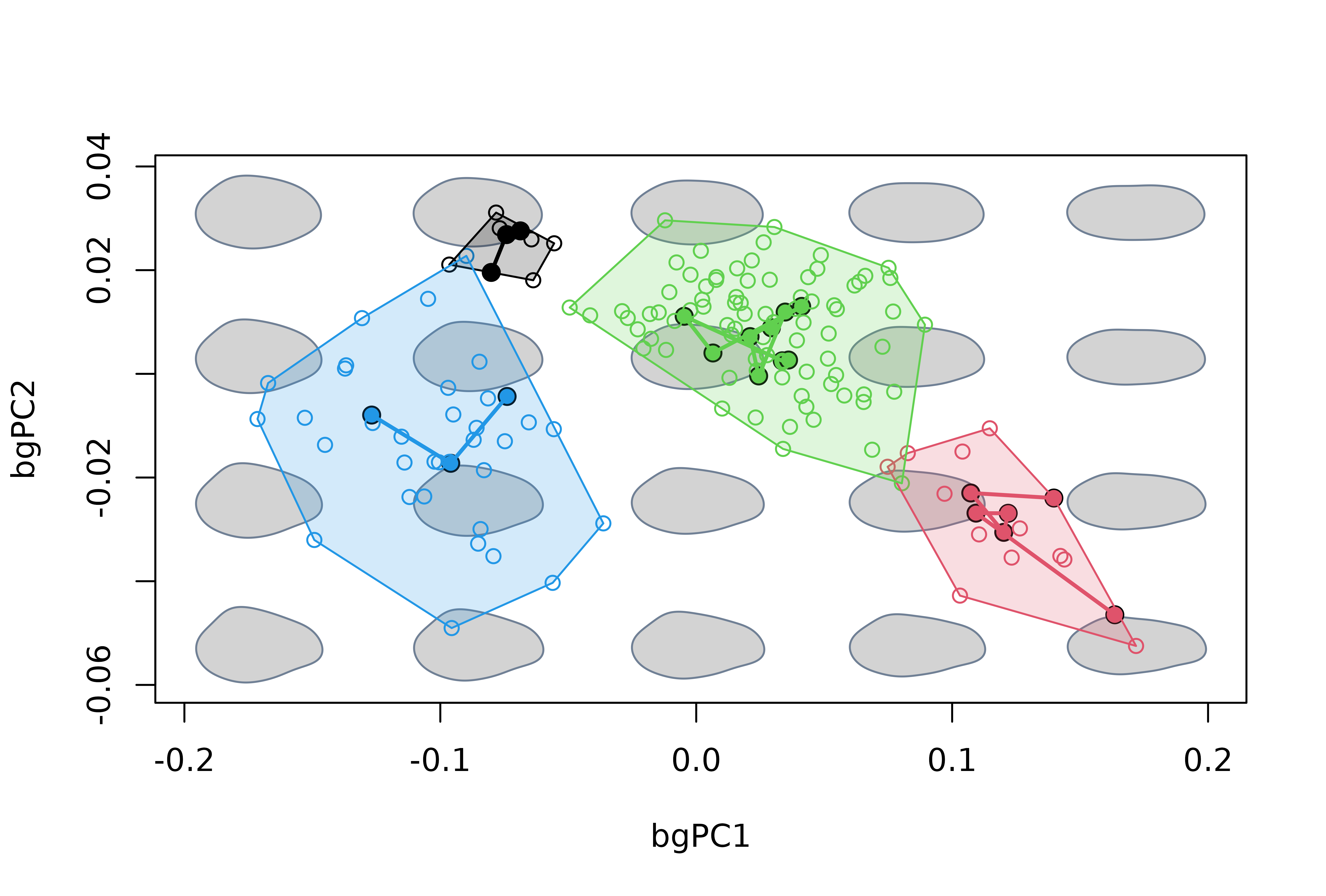Finally, we use plot_mspace to plot geochronologic age against shape. To add lines connecting the mean shape of each combination of species and biozone, we first bind them as columns, order them, and use a for loop . This particular ‘hybrid’ morphospace is much more useful to depict species’ mean morphological changes through time.

# Another visualization (probably better to interpreting temporal patterns): 
# plot time axis vs first bgPC
plot_mspace(msp, x = c(mean_ages, ages), groups = FALSE)
#> Warning in morphogrid(ordination = ordination, axes = args$axes, datype =
#> mspace$ordination$datype, : x or y has been specified, axes[2] will be ignored

# Combine 1) scores corresponding to mean shapes and 2) mean ages for each 
# level of species:biozone 
xy <- cbind(mean_ages, msp$projected$scores[1:nlevels(sp.bz), 1])
xy <- xy[order(xy[,1]),]

# Add anagenetic trajectories in 'stratomorphospace'
for(i in 1:nlevels(species)) {
  index <- grepl(x = rownames(xy), pattern = levels(species)[i])
  lines(xy[index,], col = i, lwd = 2)
}
title(' "Stratomorphospace" ')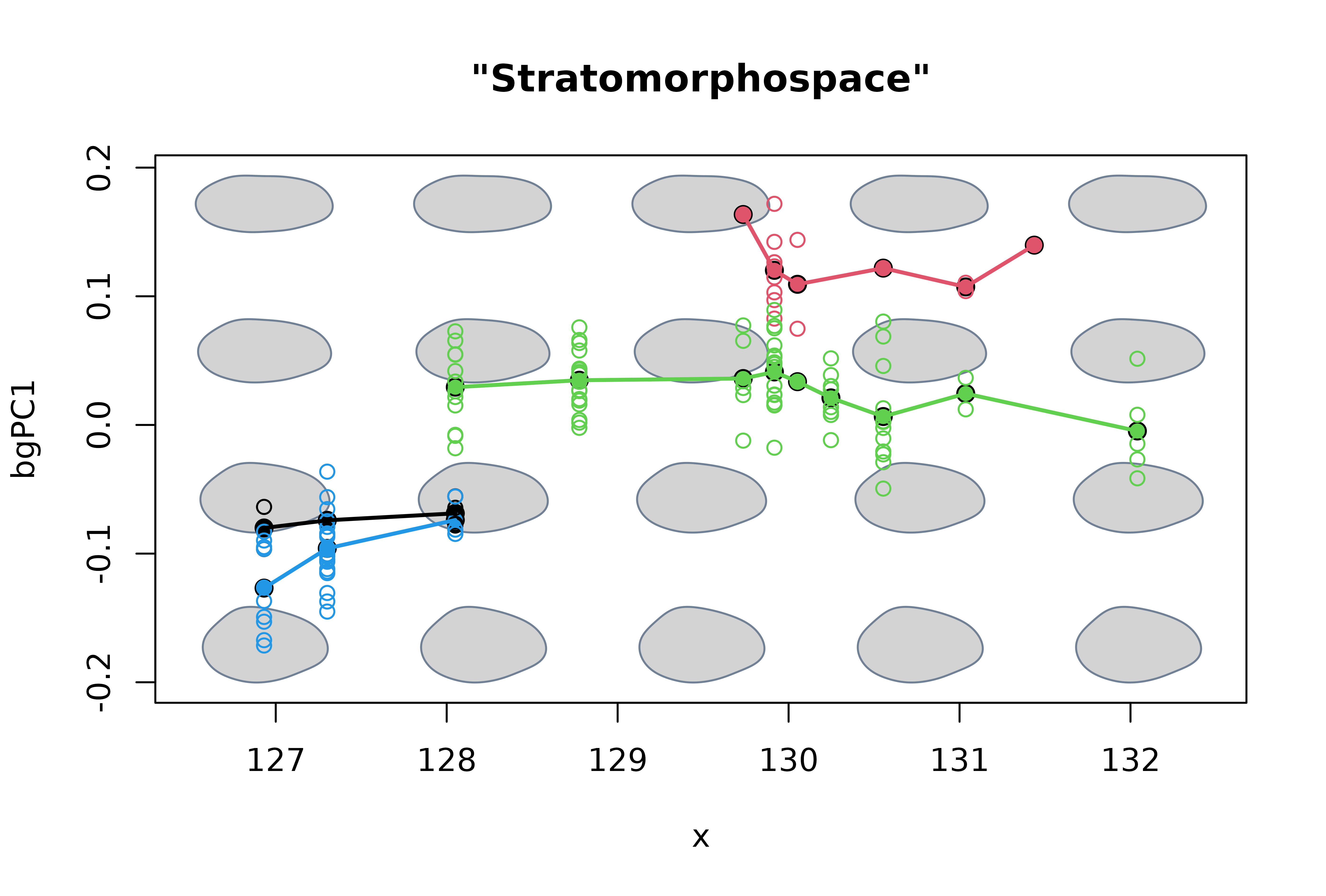

From these plots we can say that, regarding the shell outline, 1) P esbelta is rather different from the rest of the species, 2) P coihuicoensis and P. windhauseni are very similar to each other, and 3) most of the species show little or no net change over their stratigraphic span (in other words they seem to be under morphological stasis), with the exception of P. windhauseni which shows a short but noticeable directional trend towards higher shells.

3D Landmark data

Last but not least, morphospace can also deal with 3D landmark data (my personal preference for importing and normalizing 3D landmark data are the functions from Morpho, but other packages can do this too). To show how to apply the mspace %>% proj_* workflow we use the shells3D data set taken from Milla Carmona et al. (2021), which gathers longitudinal ontogenetic data from 67 specimens belonging to 7 species of the extinct bivalve genus Steinmanella from the Lower Cretaceous of Argentina. The shape of these specimens was registered at different sizes using growth lines, and so the data set includes a total of 278 shapes quantified using 90 surface semilandmarks. Also included are the corresponding centroid sizes, the id of the specimen each shape was taken from, and information about biostratigraphic age, taxonomic classification and geographic provenance of each specimen. The surface mesh corresponding to the specimen closest to the consensus of the sample (found using geomorph::findMeanSpec) is also included.

The rgl package (Murduch & Adler 2021) is responsible for depiction of 3D models, which imposes some important differences in the way morphospace functions work. Most importantly, each time mspace or plot_mspace is called, a rgl device will pop up and the user will be asked to rotate a reference shape to a desired orientation. Do not close or minimize this window, just expand it and/or rotate and zoom in/out the model and then go to the console and hit Enter there directly.

We start by loading the relevant packages and set a rotation matrix for rgl models (you wouldn’t normally need this step, but because I since cannot rotate the device when knitting this becomes necessary. However it can also be useful to use it in your workflow too, so you don’t need to worry about finding exactly the same orientation over and over again.)

# Load packages
library(geomorph)
library(magrittr)
library(Morpho)
library(morphospace)
library(rgl)


# Set a rotation matrix
par3d(userMatrix = 
        matrix(c(-0.92221391,-0.37156740,-0.10704762,0,-0.37703809,
                 0.92551011,0.03568961,0,0.08581252,0.07327446,
                 -0.99361324,0,0,0,0,1), nrow = 4, ncol = 4, byrow = TRUE)
)

# Load data from 3D shells, extract shapes and classification into species
data("shells3D")

shapes <- shells3D$shapes
sizes <- log(shells3D$sizes)
species <- shells3D$data$species
ind <- shells3D$data$individual
bzones <- shells3D$data$biozone
locality <- shells3D$data$locality
mesh_meanspec <- shells3D$mesh_meanspec

# compute consensus of each species
sp_shapes <- expected_shapes(shapes, species)

# Pile shapes
pile_shapes(shapes, alpha = 0.2)

# Create morphospace using raw variation. This is interactive, 
# you need to rotate the 3D model by yourself and then press 
# enter into the console
mspace(shapes, cex.ldm = 2, adj_frame = c(0.9, 0.85), plot = TRUE) %>%
  proj_shapes(shapes = shapes, bg = species, pch = 21) %>%
  proj_groups(shapes = shapes, groups = species, ellipse = TRUE, alpha = 0.2) %>%
  proj_shapes(sp_shapes, pch = 21)
title("Morphospace")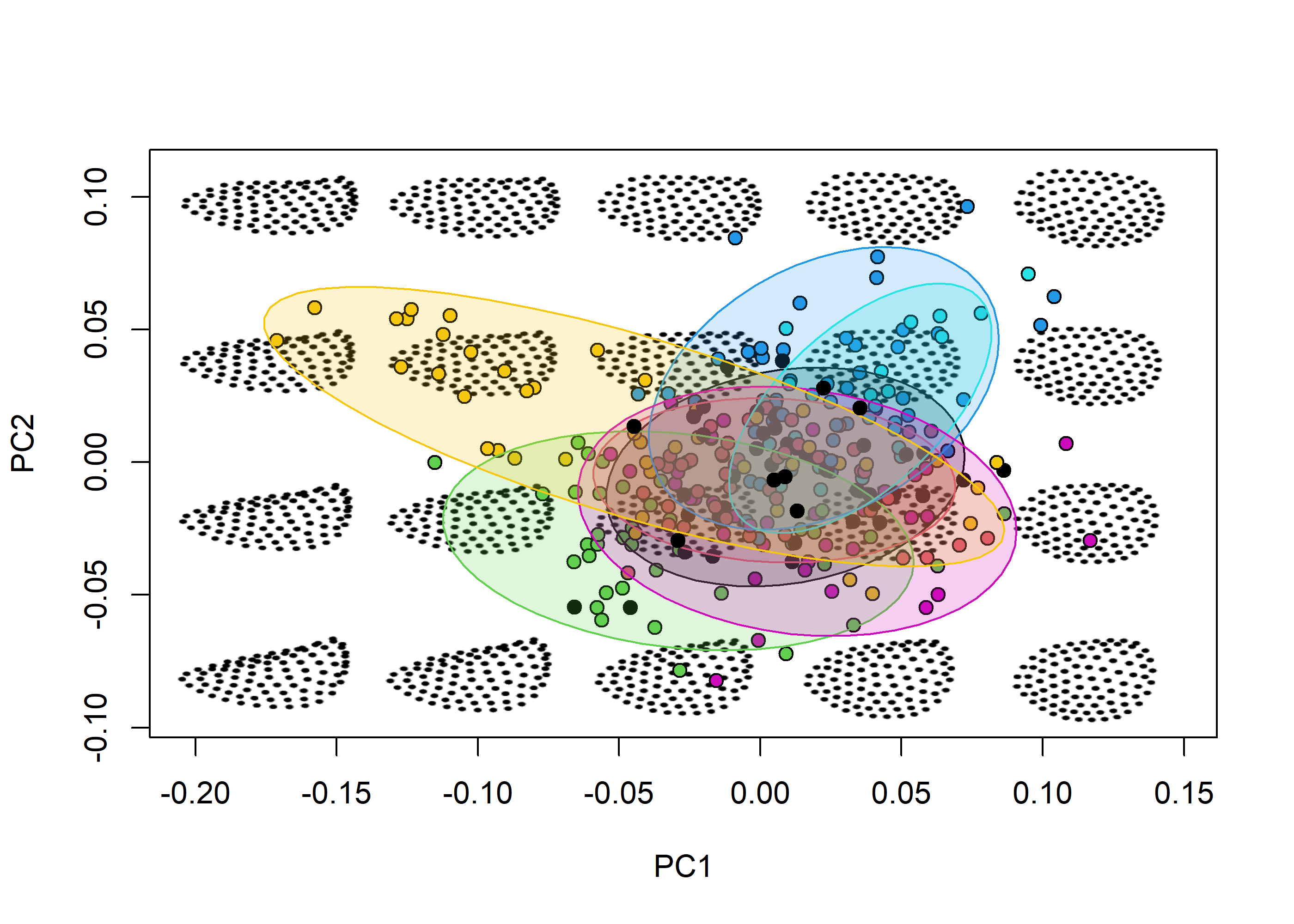

We can now focus on ontogenetic shape variation, which was the purpose this data set was built for. Again we resort to detrend shapes to remove variation introduced by undesired sources (which in this case are biostratigraphic level, geographic provenance and, especialy, individual differences).

# Remove nuisance variation from the sample, for each species 
# (a couple were registered in a single biozone and/or locality, 
# which require little adjustments)
detr_shapes <- shapes * 0
for(i in 1:nlevels(species)) {
  index <- species == levels(species)[i]
  subshapes_mat <- two.d.array(shapes[,,index])
  subind <- ind[index]
  subloc <- locality[index]
  subzone <- bzones[index]

  if(!any(i == c(4, 5))) {
    detr_shapes[,,index] <- lm(subshapes_mat ~ subind * subzone * subloc) %>%
      detrend_shapes(method = "residuals") %>% arrayspecs(p = 90, k = 3)
  } else {
    if(i == 4) {
      detr_shapes[,,index] <- lm(subshapes_mat ~ subind) %>%
        detrend_shapes(method = "residuals") %>% arrayspecs(p = 90, k = 3)
    } else {
      detr_shapes[,,index] <- lm(subshapes_mat ~ subind * subloc) %>%
        detrend_shapes(method = "residuals") %>% arrayspecs(p = 90, k = 3)
    }
  }
}

As with 2D landmarks we can include a template to improve interpretability, although in this case this template is a 3D surface mesh. This can slow down the process a bit, especially if we ask for too many models, use transparent meshes, or use LOOCV. The template used must be the mesh corresponding to the mean shape of the sample, which needs to be computed beforehand (the shells3D data set includes the mesh corresponding to the specimen closest to the consensus, which can be warped using Morpho::tps3d to obtain the mean mesh, as shown in the next chunk).

# Generate morphospace using raw variation, but with a mesh template that 
# improves visualization:

# First, get shape corresponding to shells3D$mesh_meanspec using 
# geomorph::findMeanSpec,
meanspec_id<- findMeanSpec(shapes)
meanspec_shape <- shapes[,,meanspec_id]


# Then get consensus shape and warp the mean spec mesh to get the mesh 
# corresponding to the consensus using Morpho::tps3d
detr_meanshape <- expected_shapes(detr_shapes)
detr_meanmesh <- tps3d(x = mesh_meanspec, refmat = meanspec_shape, 
                       tarmat = detr_meanshape)

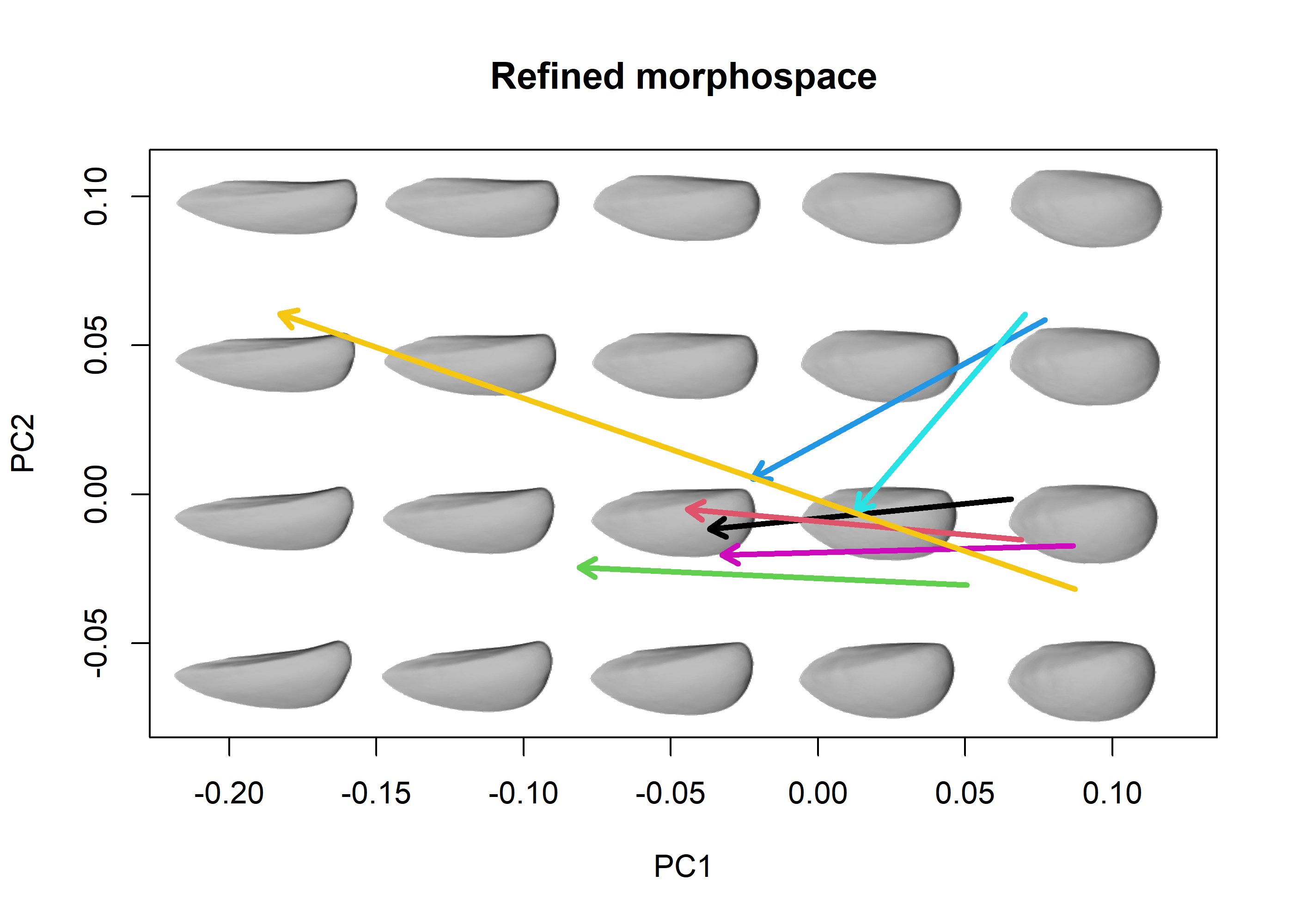
Once we got rid of the noise and have our template prepared, we use the refined shapes to compute the ontogenetic allometric axis of each species using pls_shapes. Then, we use the former to generate a morphospace in which to project the latter, using 3D meshes as background shape models.

# Compute allometric axis of each species using pls_shapes
pls_list <- lapply(1:nlevels(species), function(i) {
  index <- species == levels(species)[i]
  subshapes <- detr_shapes[,,index]
  subsizes <- sizes[index]

  pls_shapes(shapes = two.d.array(subshapes), X = subsizes, LOOCV = TRUE)

})


# Generate morphospace from refined variation and project allometric
# axis, add legend
allomsp <- mspace(detr_shapes, template = detr_meanmesh, bg.model = "gray",
                  cex.ldm = 0, invax = 1, adj_frame = c(0.9, 0.85)) %>%
  proj_shapes(shapes = detr_shapes, cex = 0, col = species)
title("Refined morphospace")

# use proj_axis outside the pipeline with pipe = FALSE
for(i in 1:nlevels(species)) {
  proj_axis(mspace = allomsp, obj = pls_list[[i]], lwd = 3, col = i, 
            type = 2, axis = 1, pipe = FALSE)
}

We can use plot_mspace to plot an allometric axis (represented by the axis resulting from the PLS of shape and size of the entire sample). In order to improve interpretation of results, we will first use expected_shapes to compute the shape expected for each size by the linear regression of the latter on the former (we do this species-wise), to be projected into the allometric axis. Then, we call plot_mspace, including 1) the "mspace" object built with PLS (indicating the first and only axis with axes = 1), 2) the size variable using x, and 3) a legend with legend = TRUE.

# Compute shapes expected under the linear relationship of size and shape. The
# code below will apply expected_shapes to the shapes and sizes of each species,
# rearrange them as an array, and reorder them according to their original order
pred_shapes <- abind::abind(
  lapply(1:nlevels(species), function(i) {
    index <- species == levels(species)[i]
    subshapes <- detr_shapes[,,index]
    subsizes <- sizes[index]
    
    expected_shapes(shapes = subshapes, x = subsizes)
  }), 
  along = 3)[,,dimnames(shapes)[[3]]]

# Then create allomorphospace using PLS to emphasize allometric variation 
# (this could take a moment due to the leave-one-out cross-validation) and
# project the expected shapes (with point sizes proportional to each specimen's
# original size) as well as the species classification (this last thing is
# necessary for adding a legend):
allomsp2 <- mspace(detr_shapes, FUN = pls_shapes, X = sizes, LOOCV = TRUE,
                   bg.model = "gray", cex.ldm = 0, template = detr_meanmesh, 
                   invax = 1, plot = FALSE) %>% 
  proj_shapes(pred_shapes, pch = 21, bg = species, cex = (sizes/max(sizes))^3) %>% 
  proj_groups(groups = species)


# Finally, use plot_mspace to create hybrid morphospace with shape against 
# Size, and add legend
plot_mspace(allomsp2, x = sizes, axes = 1, xlab = "log-size", 
            adj_frame = c(0.9, 0.85), groups = FALSE, legend = TRUE)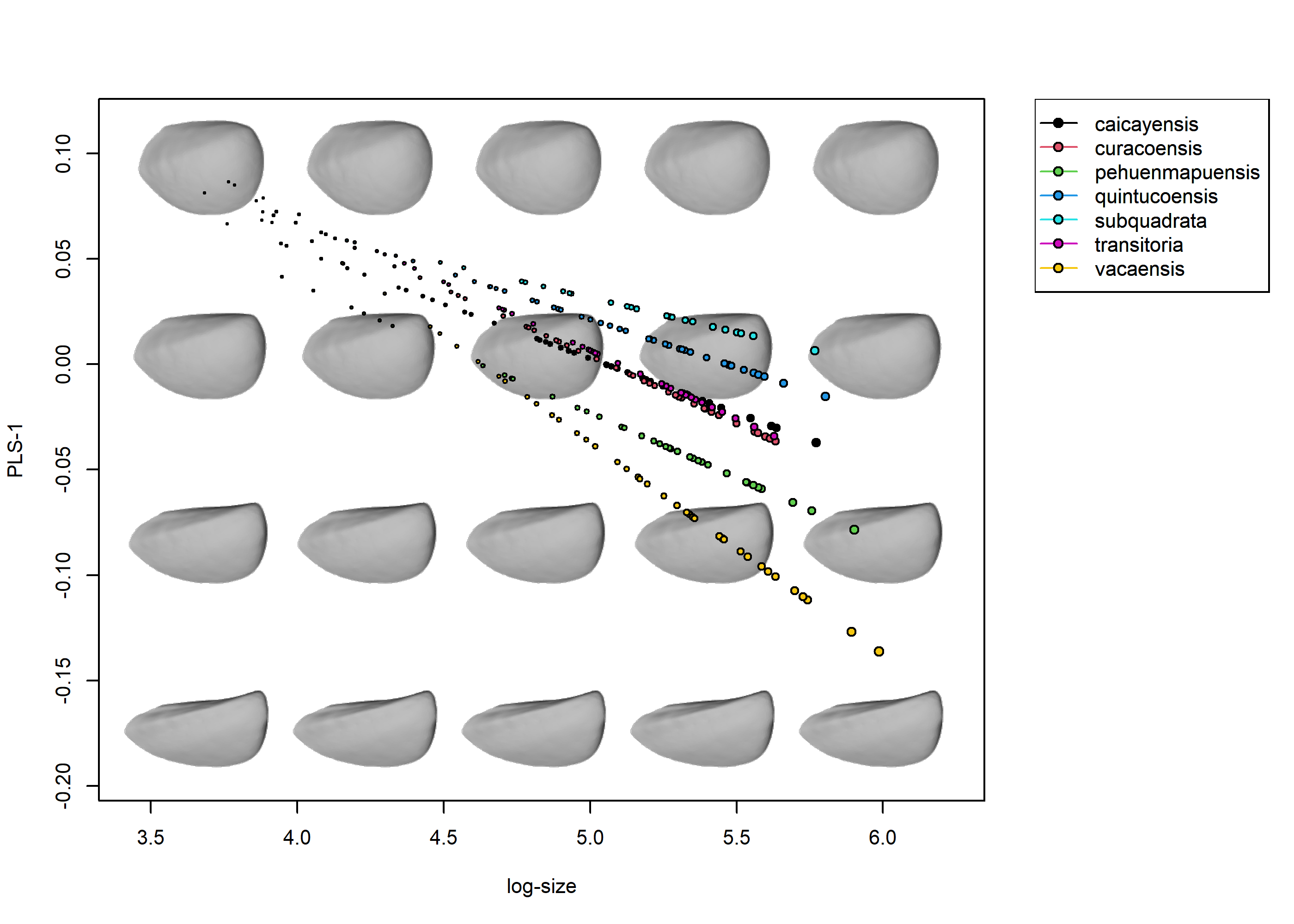

A quick assessment of these plots tells us that there are two main groups of ontogenies: those from S. quintucoensis and S. subquadrata (which go from roughly quadrate shells with expanded posteriors to more rectangular shells) and the rest of the species, whose ontogenetic trajectories seem to be very similar in terms of orientation and magnitude (all of them go from more oval-like shells to more triangular ones, although the position of the trajectory differs). The exception is S. vacaensis, which show a protracted trajectory which reach some very elongated shell shapes. It is also apparent that the common trend is one of anteroposterior elongation, which seems to be more marked for the two species reaching larger sizes (S. pehuenmapuensis and S. vacaensis).

References

Milla Carmona P.S, Lazo D.G., & Soto I.M. (2018). Morphological evolution of the bivalve Ptychomya through the Lower Cretaceous of Argentina. Paleobiology, 44(1), 101-117 https://doi.org/10.1017/pab.2017.32.

Milla Carmona P.S, Lazo D.G., & Soto I.M. (2021). Ontogeny in the steinmanellines (Bivalvia: Trigoniida): an intra- and interspecific appraisal using the Early Cretaceous faunas from the Neuquén Basin as a case study. Paleobiology, in press. https://doi.org/10.1017/pab.2021.32.

Murdoch D., & Adler D. (2021). rgl: 3D Visualization Using OpenGL. R package version 0.108.3. https://cran.r-project.org/package=rgl.

Soto E.M., Goenaga J., Hurtado J.P., & Hasson E. (2012). Oviposition and performance in natural hosts in cactophilic Drosophila. Evolutionary Ecology, 26, 975-990. https://doi.org/10.1007/s10682-011-9531-5