Remove shape variation associated to external variables

Detrend shape variation using the relationship between shape data and some external explanatory variable(s) (works for both factors and numerics).

detrend_shapes(
  model,
  xvalue = NULL,
  tree = NULL,
  method = "orthogonal",
  newdata = NULL
)

Arguments

model: A "mlm" object created using stats::lm().
xvalue: A value (numeric) or level (character) at which shape data is to be standardized (i.e., centered); If NULL, the mean of the complete sample is used (only available if there is a single explanatory variable).
tree: A "phylo" object containing a phylogenetic tree. Tip labels should match row names from x.
method: Method used for detrending; options are "orthogonal" (the default) and "residuals" (see details).
newdata: New data to be standardized. It should be provided as either an "mlm" object fitting the same variables used in model measured in a new sample, created through stats::lm(), or a 2-margin matrix of shape descriptors (only for method = "orthogonal"). See details.

Value

A 2-margins matrix, of dimensions n x (k x p) for the case of landmark data and n x (4 x nb.h) for the case of Fourier data (where nb.h is the number of harmonics used in elliptic Fourier analysis).

Details

This function detrends (or standardizes, or corrects) shapes from variation associated with non-shape variables, using either the residuals computed from a linear model fitting the former to the latter (method = "residuals"), or the projection of shapes into a subspace that is orthogonal to variation associated to non-shape variables, computed using the Burnaby approach (method = "orthogonal").

If newdata is provided as an "mlm" object, shapes from newdata are detrended by "correcting" their relationship with the explanatory variables using the relationship estimated for the data provided in model ("partial detrending"). Specifically, if method = "residuals", shape residuals will be computed by subtracting values fitted to the coefficients from model to the shapes provided in newdata; whereas if method = "orthogonal", shapes are projected into the subspace resulting from the subtraction of the orthogonal subspaces computed for newdata and model.

If method = "orthogonal" and newdata is provided as a 2-margin matrix of shape descriptors, the function will instead return the new set of shapes, detrended using the relationship estimated for the data provided in model (i.e., the shapes provided in newdata are projected directly into the orthogonal subspace computed for the data provided in model).

The grand mean of the sample of shapes is used by default to center shape variation, although an xvalue specifying a level or numeric value of the explanatory variable in model to center shapes at can be provided. This shift can only be applied for one explanatory variable.

If a phylogenetic tree is supplied for interspecific shape data, the procedure is performed using the phylogenetically-corrected coefficients (and the phylogenetic mean is used instead of the grand mean for re-centering data; see Revell, 2009), assuming a Brownian motion model of evolution.

References

Burnaby, T. P. (1966) Growth-invariant discriminant functions and generalized distances. Biometrics, 22, 96–110.

Revell, L. J. (2009). Size-correction and principal components for interspecific comparative studies. Evolution, 63, 3258-3268.

Klingenberg, C. P. (2016). Size, shape, and form: concepts of allometry in geometric morphometrics. Development Genes and Evolution, 226(3), 113-137.

Examples

 #### Landmark data

 #load tails data and packages
 library(geomorph)
 library(Morpho)

 data(tails)
 shapes <- tails$shapes
 species <- tails$data$species
 sex <- tails$data$sex
 logsizes <- log(tails$sizes)
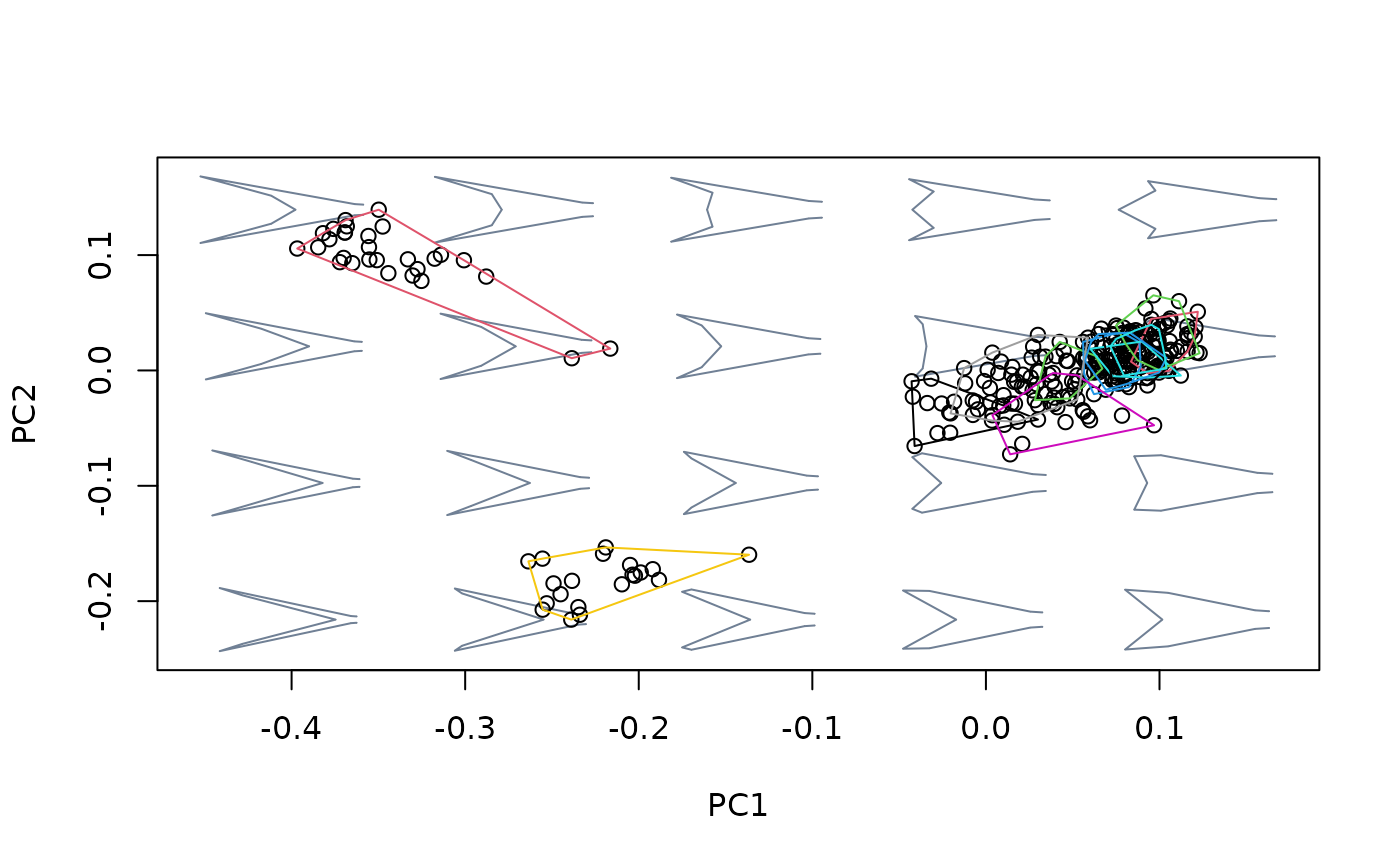
 msp <- mspace(shapes, links = tails$links, points = TRUE)
 hulls_by_group_2D(msp$ordination$x, fac = species)



 ### For numeric variables

 #fit linear model between shapes and sizes, then center at the grand mean of
 #the sample
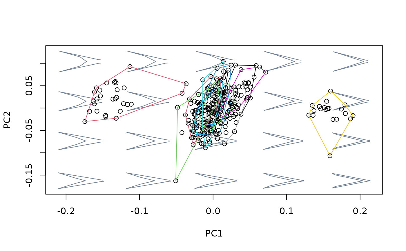
 model <- lm(two.d.array(shapes) ~ logsizes)
 detr_shapes_mat <- detrend_shapes(model)

 detr_shapes_nosize <- arrayspecs(detr_shapes_mat, k = 2, p = 9)

 msp_nosize <- mspace(detr_shapes_nosize, links = tails$links, points = TRUE)
 hulls_by_group_2D(msp_nosize$ordination$x, fac = species)


 ## Using xvalue

 #fit linear model between shapes and sizes, then center at the shape
 #corresponding to the maximum size of the sample
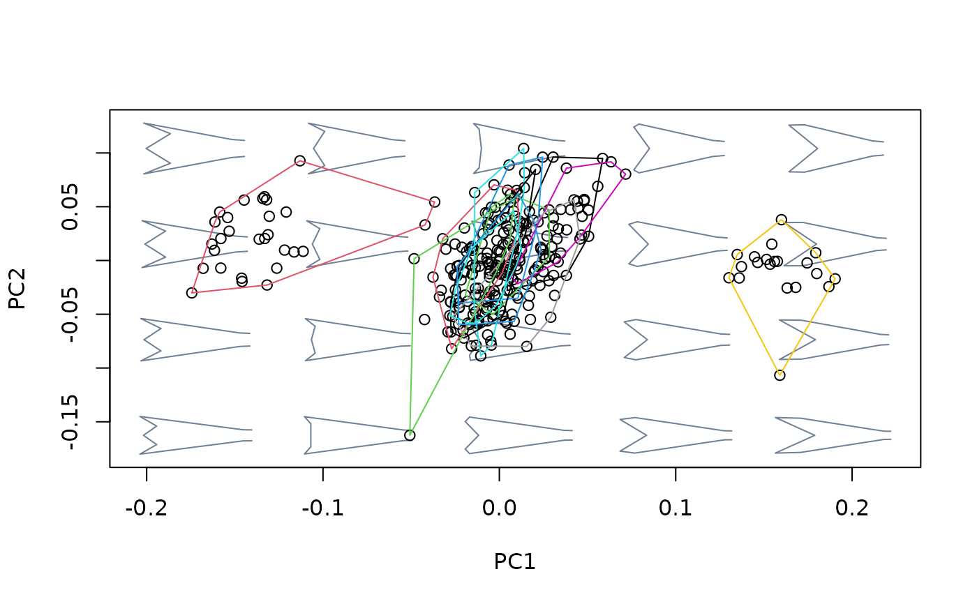
 model <- lm(two.d.array(shapes) ~ logsizes)
 detr_shapes_mat2 <- detrend_shapes(model,
                                    xvalue = max(logsizes))

 detr_shapes_nosize2 <- arrayspecs(detr_shapes_mat2, k = 2, p = 9)

 msp_nosize2 <- mspace(detr_shapes_nosize2, links = tails$links,
                       points = TRUE)
 hulls_by_group_2D(msp_nosize2$ordination$x, fac = species)


 ## Using a phylogenetic tree

 #fit linear model between shapes and sizes, then center at the shape
 #corresponding to the grand size of the sample
 sp_shapes <- expected_shapes(shapes, species)
 sp_logsizes <- c(tapply(logsizes, species, mean))
 model <- lm(two.d.array(sp_shapes) ~ sp_logsizes)
 detr_shapes_mat1 <- detrend_shapes(model)

 detr_shapes_nosize1 <- arrayspecs(detr_shapes_mat1, k = 2, p = 9)

 msp_nosize1 <- mspace(detr_shapes_nosize1, links = tails$links,
                       points = TRUE)
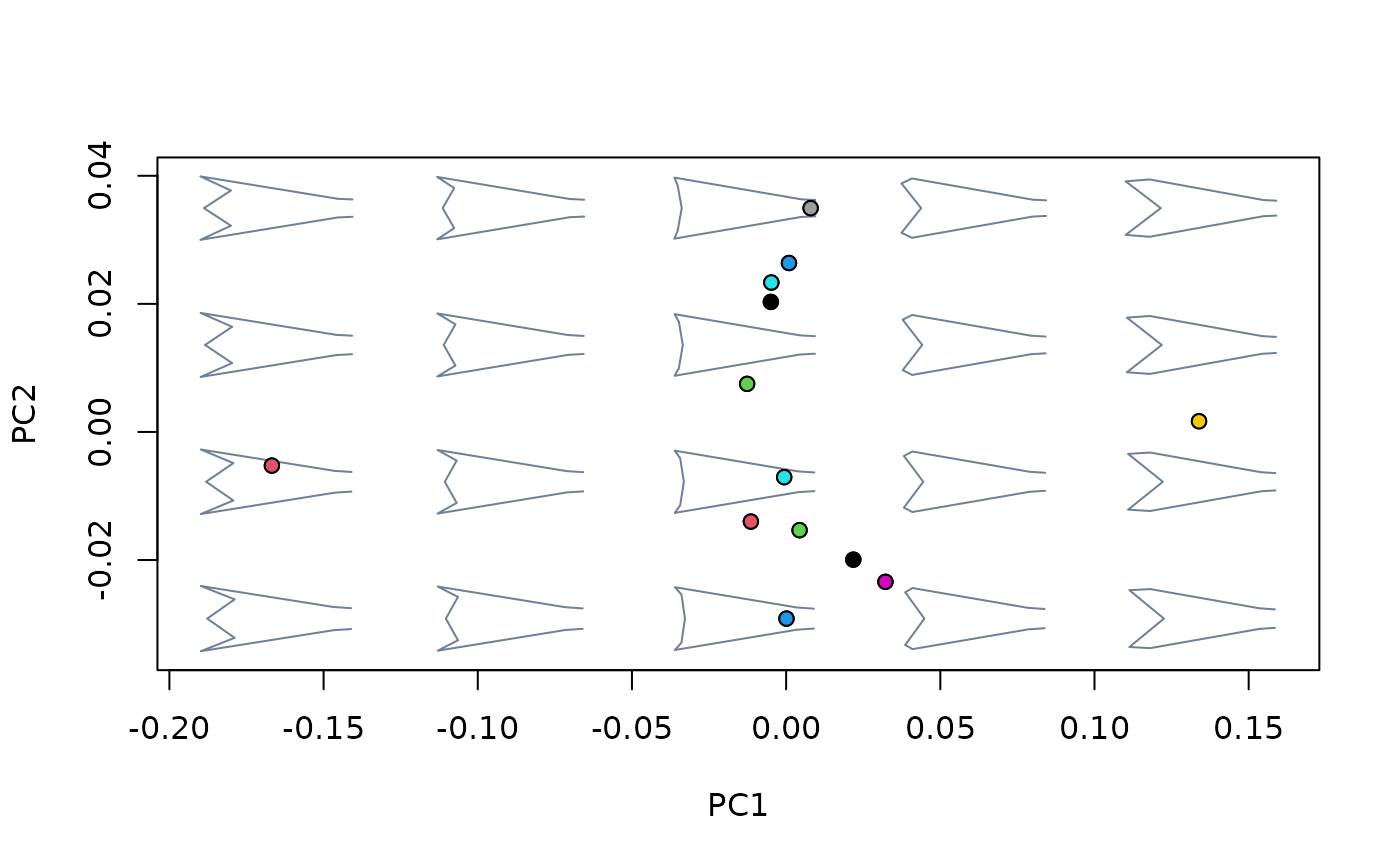
 points(msp_nosize1$ordination$x, pch = 21, bg = c(1:13))


 ## Using newdata

 #fit linear model between shapes and sizes for NDF species, then use the NDF
 #allometry to detrend DF shapes from allometric variation (just for
 #illustration, not implying this makes any sense)
 index <- tails$data$type == "NDF"
 shapes_ndf <- shapes[,,index]
 logsizes_ndf <- logsizes[index]
 shapes_df <- shapes[,,!index]
 logsizes_df <- logsizes[!index]

 model_ndf <- lm(two.d.array(shapes_ndf) ~ logsizes_ndf)
 model_df <- lm(two.d.array(shapes_df) ~ logsizes_df)
 detr_shapes_mat3 <- detrend_shapes(model_ndf, newdata = model_df)

 detr_shapes_nosize3 <- arrayspecs(detr_shapes_mat3, k = 2, p = 9)

 msp_nosize3 <- mspace(detr_shapes_nosize3, links = tails$links,
                       points = TRUE)
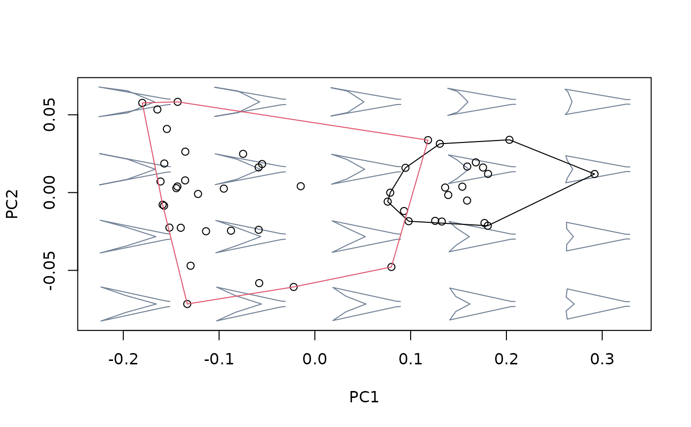
 hulls_by_group_2D(msp_nosize3$ordination$x, fac = factor(species[!index]))


 ### For factors

 #load wings data

 data(wings)
 shapes <- wings$shapes
 cactus <- wings$data$cactus
 sex <- wings$data$sex
 species <- wings$data$species
 msp <- mspace(shapes, template = wings$template, points = TRUE)
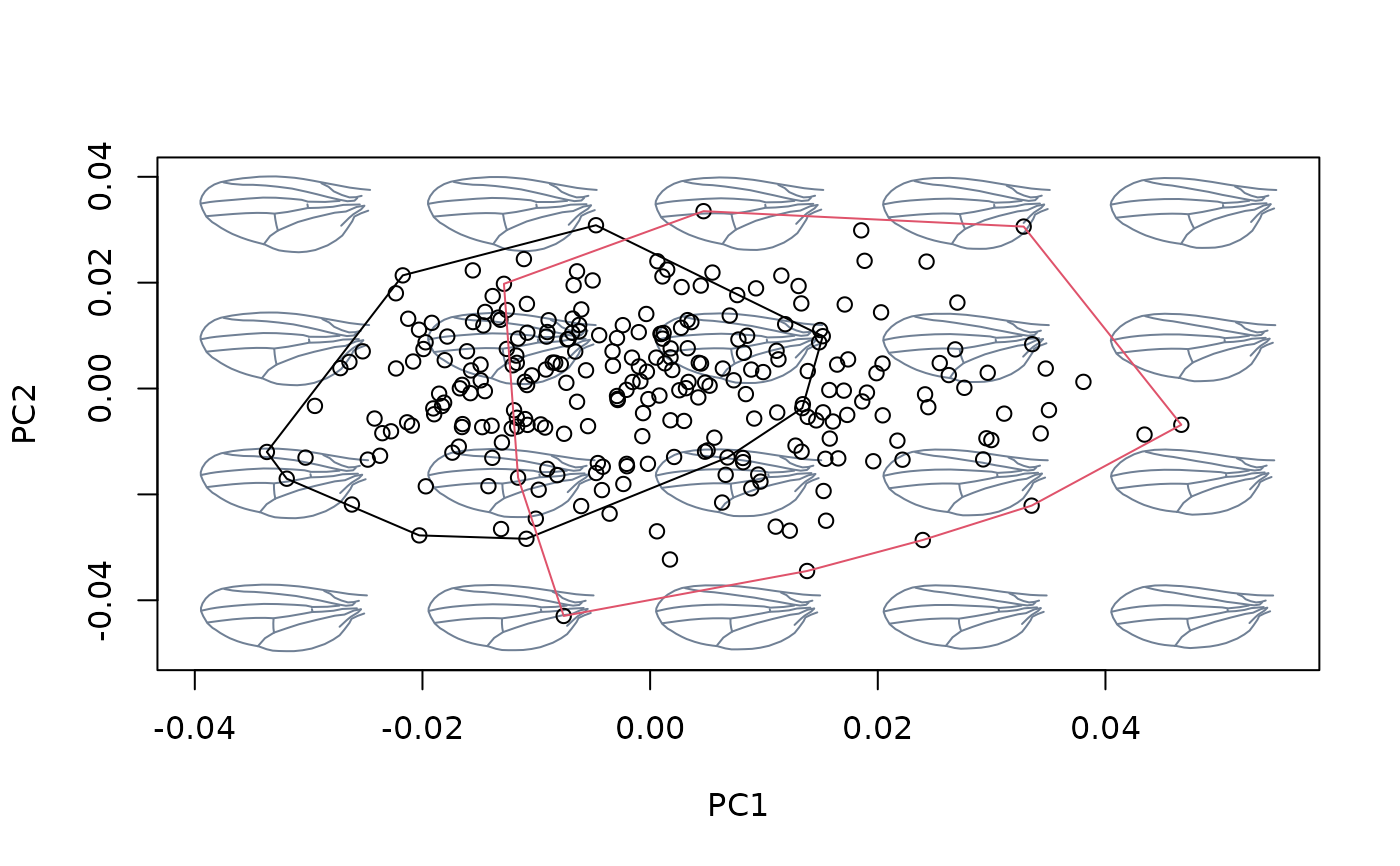
 hulls_by_group_2D(msp$ordination$x, fac = cactus)



 #fit linear model between shapes and sex, then center at the grand mean
 #of the sample.
 model <- lm(two.d.array(shapes) ~ cactus)
 detr_shapes_mat <- detrend_shapes(model)

 detr_shapes_nocac <- arrayspecs(detr_shapes_mat, k = 2, p = 9)

 msp_nocac <- mspace(detr_shapes_nocac, template = wings$template,
                     points = TRUE)
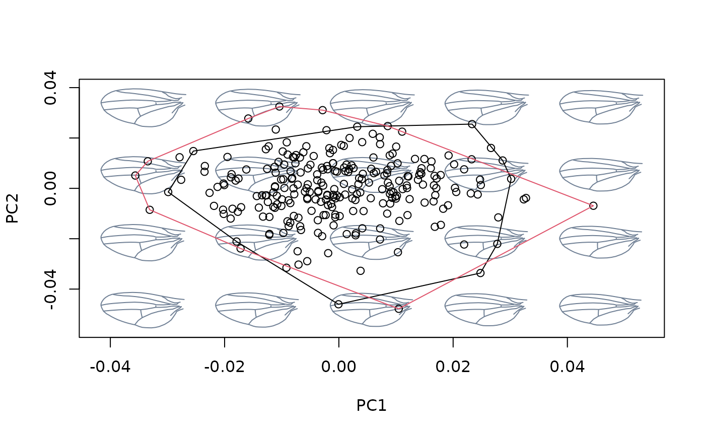
 hulls_by_group_2D(msp_nocac$ordination$x, fac = cactus)


 ## Using xvalue

 #fit linear model between shapes and species, then center at the shape
 #corresponding to the mean shape of T. savana
 model <- lm(two.d.array(shapes) ~ cactus)
 detr_shapes_mat <- detrend_shapes(model, xvalue = "Tr")

 detr_shapes_nocac2 <- arrayspecs(detr_shapes_mat, k = 2, p = 9)

 msp_nocac2 <- mspace(detr_shapes_nocac2, template = wings$template,
                      points = TRUE)
 hulls_by_group_2D(msp_nocac2$ordination$x, fac = cactus)


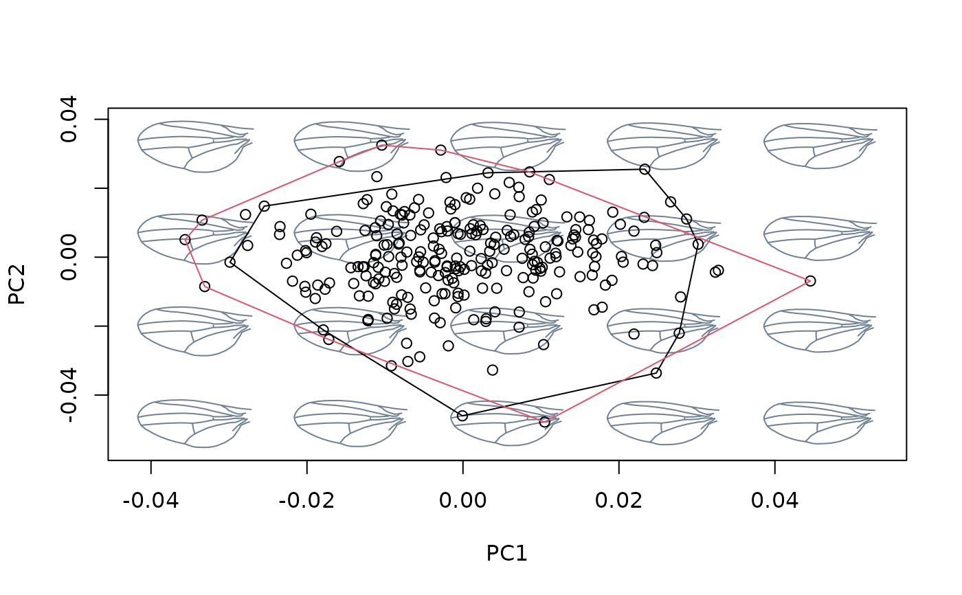 ## Using newdata

 #fit linear model between shapes and cactus for Db species, then use this
 #relationship to detrend Dk shapes from variation between cactus
 index <- species == "Db"
 shapes_Db <- shapes[,,index]
 cactus_Db <- cactus[index]
 shapes_Dk <- shapes[,,!index]
 cactus_Dk <- cactus[!index]

 model_Db <- lm(two.d.array(shapes_Db) ~ cactus_Db)
 model_Dk <- lm(two.d.array(shapes_Dk) ~ cactus_Dk)
 detr_shapes_mat3 <- detrend_shapes(model_Db, newdata = model_Dk)

 detr_shapes_nocactus <- arrayspecs(detr_shapes_mat3, k = 2, p = 9)

 msp_cactus <- mspace(shapes_Dk, template = wings$template, points = TRUE)
 hulls_by_group_2D(msp_cactus$ordination$x, fac = factor(cactus[!index]))


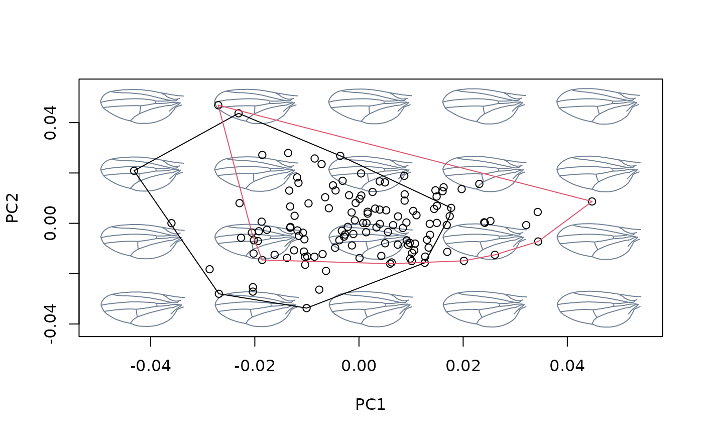 msp_nocactus <- mspace(detr_shapes_nocactus, template = wings$template,
                     points = TRUE)
 hulls_by_group_2D(msp_nocactus$ordination$x, fac = factor(cactus[!index]))



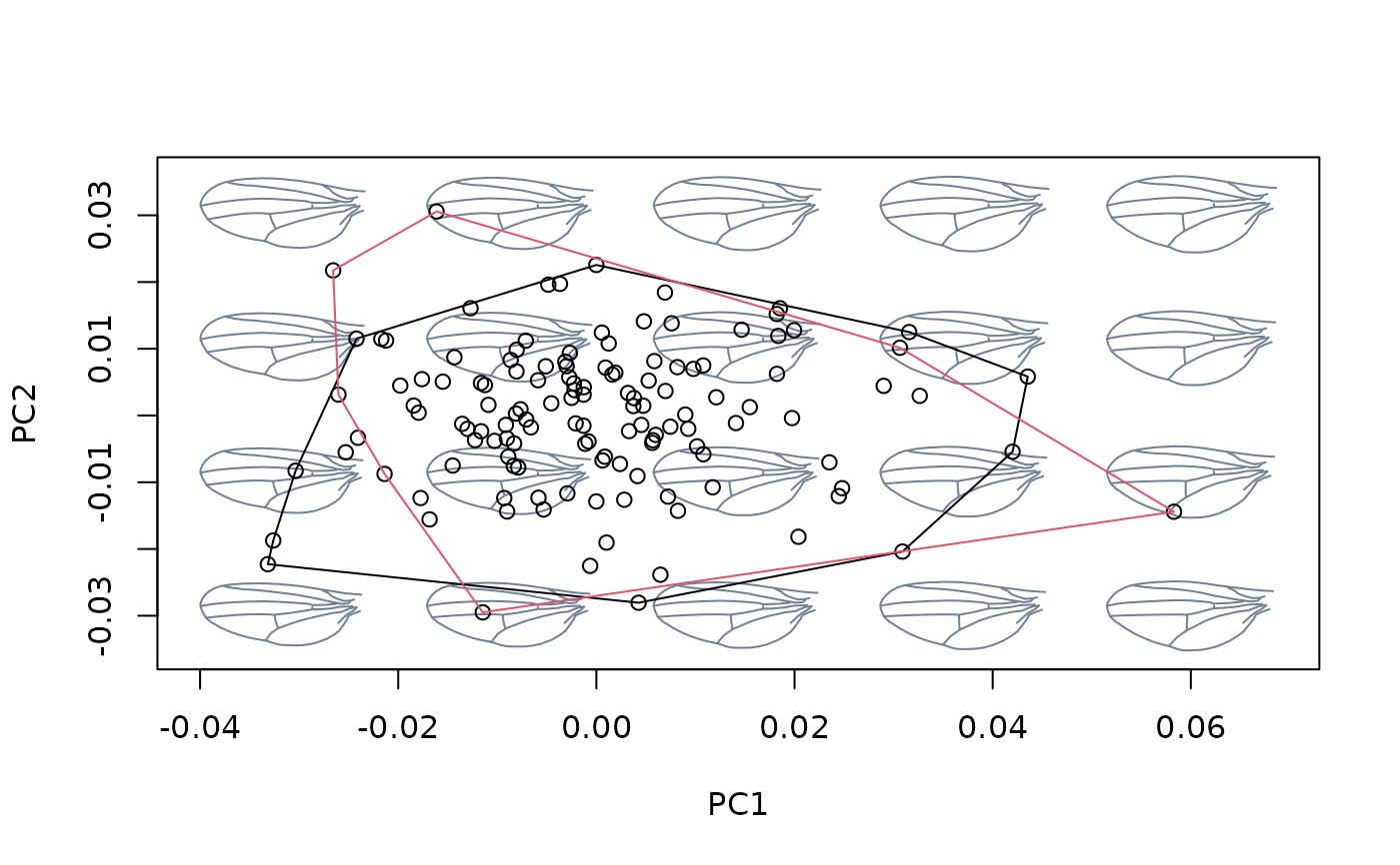 ### Comparing residuals vs orthogonal methods

 if (FALSE) {
 #load shells3D data, retain only specimens belonging to S. vacaensis
 data("shells3D")
 index <- species == levels(species)[7]
 shapes <- shells3D$shapes
 refmesh <- shells3D$mesh_meanspec
 species <- shells3D$data$species
 sizes <- log(shells3D$sizes)
 template <- Morpho::tps3d(x = refmesh,
                           refmat = shapes[,,findMeanSpec(shapes)],
                           tarmat = expected_shapes(shapes[,,index]))

 #compute allometric axis (i.e., shape variation associated to changes in
 #size)
 alloax <- lm(two.d.array(shapes[,,index]) ~ sizes[index])

 #project vacaensis specimens into the overall morphospace together with
 #allometric axis
 mspace(shapes, template = template, bg.models = "gray",
        cex.ldm = 0, alpha.models = 0.7, adj_frame = c(0.93,0.93)) %>%
   proj_shapes(shapes[,,index], pch = 21, bg = 7) %>%
   proj_axis(alloax, type = 2, lwd = 2, lty = 1)

 #compute non-allometric variation using linear models (center on the shape
 #corresponding to the maximum size)
 detr_shapes_lm <- lm(two.d.array(shapes[,,index]) ~ sizes[index]) %>%
   detrend_shapes(method = "residuals", xvalue = max(sizes[index])) %>%
   arrayspecs(k = 3, p = 90)

 #visualize
 mspace(shapes, template = template, bg.models = "gray",
        cex.ldm = 0, alpha.models = 0.7, adj_frame = c(0.93,0.93)) %>%
   proj_shapes(shapes[,,index], pch = 1, col = 7) %>%
   proj_axis(alloax, type = 2, lwd = 2, lty = 1) %>%
   proj_shapes(detr_shapes_lm, pch = 21, bg = 7)

 #compute non-allometric variation using a orthogonal subspace (center on the
 #shape corresponding to the maximum size)
 detr_shapes_os <- lm(two.d.array(shapes[,,index]) ~ sizes[index]) %>%
   detrend_shapes(method = "orthogonal", xvalue = max(sizes[index])) %>%
   arrayspecs(k = 3, p = 90)

 #visualize
 mspace(shapes, template = template, bg.models = "gray",
        cex.ldm = 0, alpha.models = 0.7, adj_frame = c(0.93,0.93)) %>%
   proj_shapes(shapes[,,index], pch = 1, col = 7) %>%
   proj_axis(alloax, type = 2, lwd = 2, lty = 1) %>%
   proj_shapes(detr_shapes_os, pch = 21, bg = 7)
 }


 #### Fourier data (quick demo)

 #load shells data
 data(shells)
 shapes <- shells$shapes$coe
 species <- shells$data$species
 logsizes <- log(shells$sizes)
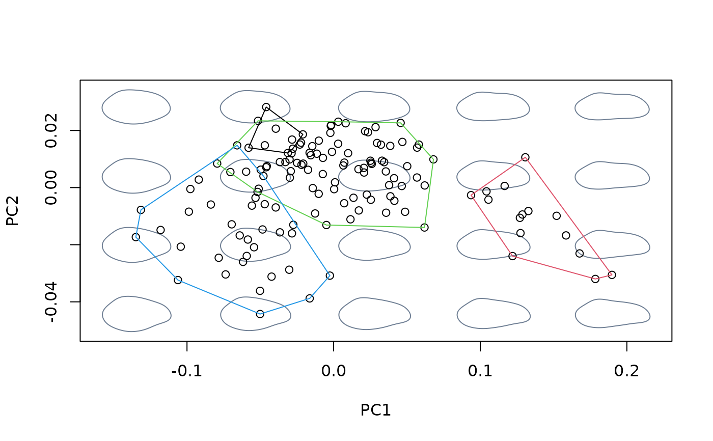
 msp <- mspace(shapes, mag = 0.5, points = TRUE)
 hulls_by_group_2D(msp$ordination$x, fac = species)


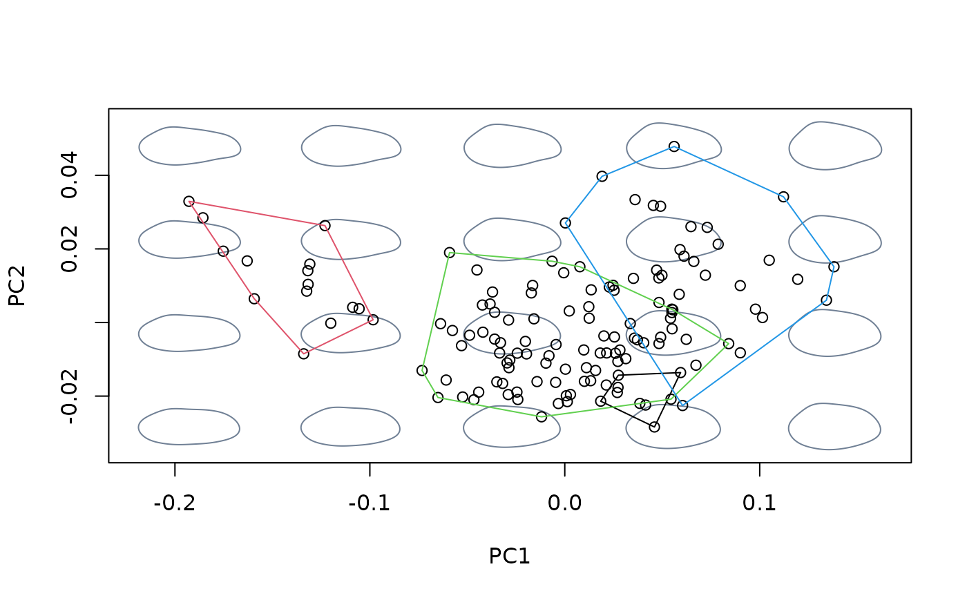 #fit linear model between shapes and sizes, then center at the shape
 #corresponding to the grand mean
 model <- lm(shapes ~ logsizes)
 detr_shapes_nosize <- detrend_shapes(model)

 msp_nosize <- mspace(detr_shapes_nosize, mag = 0.5, points = TRUE)
 hulls_by_group_2D(msp_nosize$ordination$x, fac = species)


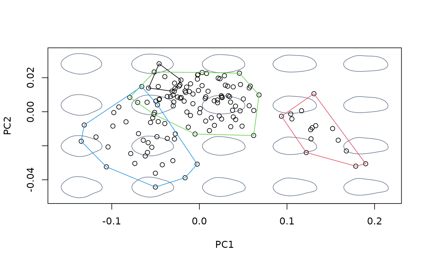
 #fit linear model between shapes and sizes, then center at the shape
 #corresponding to the maximum size
 model <- lm(shapes ~ logsizes)
 detr_shapes_nosize2 <- detrend_shapes(model,
                                       xvalue = max(logsizes))

 msp_nosize2 <- mspace(detr_shapes_nosize2, mag = 0.5, points = TRUE)
 hulls_by_group_2D(msp_nosize2$ordination$x, fac = species)


 #fit linear model between shapes and sizes, then center at the maximum size
 shapes_koeneni <- shapes[species == "koeneni",]
 logsizes_koeneni <- logsizes[species == "koeneni"]
 shapes_esbelta <- shapes[species == "esbelta",]
 logsizes_esbelta <- logsizes[species == "esbelta"]

 model_koeneni <- lm(shapes_koeneni ~ logsizes_koeneni)
 model_esbelta <- lm(shapes_esbelta ~ logsizes_esbelta)
 detr_shapes_nosize3 <- detrend_shapes(model_koeneni,
                                       newdata = model_esbelta)

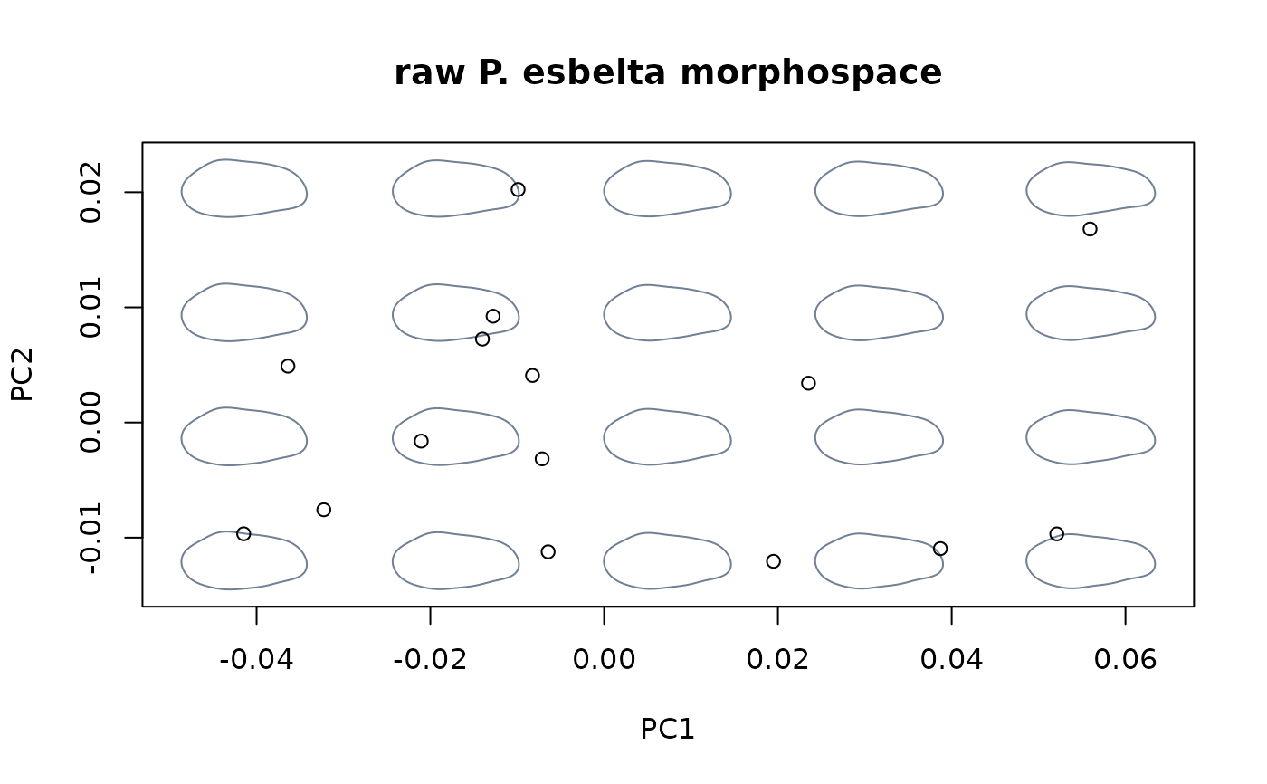
 msp_nosize3 <- mspace(shapes_esbelta, mag = 0.5, points = TRUE)
 title("raw P. esbelta morphospace")

 msp_nosize4 <- mspace(detr_shapes_nosize3, mag = 0.5, points = TRUE)
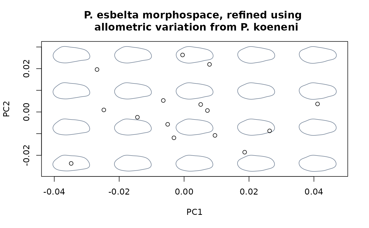
 title("P. esbelta morphospace, refined using \n allometric variation from P. koeneni")