Compute mean/expected shape(s)

Compute the mean shape from the entire sample, or the shape(s) expected for one or more levels (factors) or values (numerics) of an external explanatory variable as fitted by a linear model.

expected_shapes(
  shapes,
  x = NULL,
  xvalue = NULL,
  tree = NULL,
  returnarray = TRUE
)

Arguments

shapes

Shape data.

x

A vector or column vector containing a single explanatory variable (can be either a factor or a numeric). If NULL, the grand mean of the entire sample is computed.

xvalue

One or more numeric value(s) or factor level(s) of x at which calculate expected shape(s). If NULL, all the value(s) or level(s) are used.

tree

A "phylo" object containing a phylogenetic tree. Tip labels should match names in x and shapes.

returnarray

Logical, indicating whether shapes should be returned in "3D" array format (landmark shapes only). Mostly intended for internal use.

Value

For landmark data, either a p x k matrix defining a single mean shape or a p x k x n array containing n mean shapes, unless returnarray = TRUE (in which case a n x (p x k) matrix will be returned. For Fourier data, a n x (4 x nb.h) matrix of Fourier coefficients (with nb.h being the number of harmonics used during elliptic Fourier analysis).

Details

If a phylogenetic tree is supplied for interspecific shape data, the procedure is performed using the phylogenetically-corrected regression coefficients (see Revell, 2009) assuming a Brownian Motion model of evolution.

References

Revell, L. J. (2009). Size-correction and principal components for interspecific comparative studies. Evolution, 63, 3258-3268.

Examples

#load tails data and packages
library(Morpho)
library(Momocs)
#> 
#> Attaching package: ‘Momocs’
#> The following object is masked _by_ ‘.GlobalEnv’:
#> 
#>     wings
#> The following objects are masked from ‘package:Morpho’:
#> 
#>     export, tps2d
#> The following object is masked from ‘package:geomorph’:
#> 
#>     mosquito
#> The following object is masked from ‘package:morphospace’:
#> 
#>     wings
#> The following object is masked from ‘package:stats’:
#> 
#>     filter
data("tails")
shapes <- tails$shapes
sizes <- log(tails$sizes)
species <- tails$data$species
type <- tails$data$type
tree <- tails$tree

#compute and plot mean shape of the entire sample
mshape <- expected_shapes(shapes)
plot(mshape)
lineplot(mshape, tails$links)


#getting mean shapes for the levels of a factor: compute and plot the mean
#shape of each of the 13 species
sp_shapes <- expected_shapes(shapes, x = species)
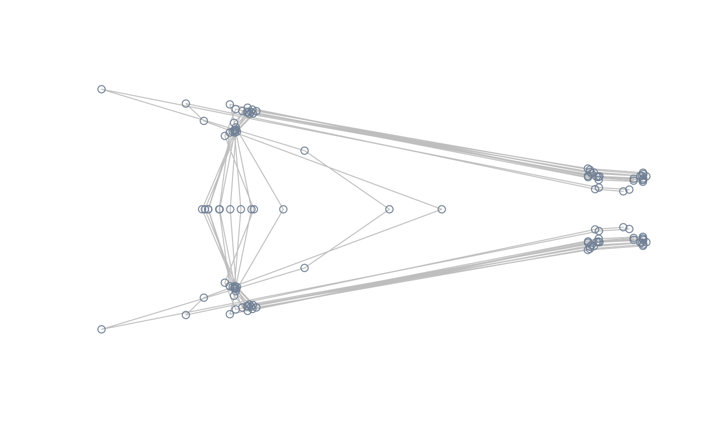
pile_shapes(sp_shapes, links = tails$links, mshape = FALSE)


#getting the mean shape for a specific level of a factor: compute and plot
#the mean shape of deep-forked specimens
df_shape <- expected_shapes(shapes, x = type, xvalue = "DF")
plot(df_shape)
lineplot(df_shape, tails$links)


#getting the mean shape for a specific level of a factor, correcting for
#phylogeny: compute and plot mean the shape of deep-forked species
sp_type <- factor(c(tapply(as.character(type), species, unique)))
df_sp_shape <- expected_shapes(sp_shapes, x = sp_type, xvalue = "DF",
                               tree = tree)
plot(df_sp_shape)
lineplot(df_sp_shape, tails$links)


#getting the shapes expected for a covariate: compute and plot the shapes
#expected under the linear regression size on of shape
exp_shapes <- expected_shapes(shapes, x = sizes)
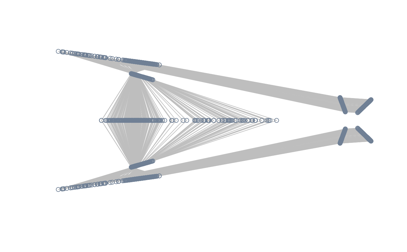
pile_shapes(exp_shapes, links = tails$links, mshape = FALSE)


#getting the shape expected for specific values of a covariate: compute and
#plot the shapes expected at the maximum size
large_shape <- expected_shapes(shapes, x = sizes, xvalue = max(sizes))
plot(large_shape)
lineplot(large_shape, tails$links)


#getting the shape expected for specific values of a covariate, correcting
#for phylogeny: compute and plot the shapes expected at the maximum size
sp_sizes <- c(tapply(sizes, species, mean))
large_sp_shape <- expected_shapes(sp_shapes, x = sp_sizes,
                                  xvalue = max(sp_sizes), tree = tree)
plot(large_sp_shape)
lineplot(large_sp_shape, tails$links)



#quick demo for Fourier data:
data("shells")
shapes <- shells$shapes

#mean shape of the entire sample
mshape <- expected_shapes(shapes)
plot(inv_efourier(mshape, nb.pts = 200), type = "l")


#mean shape of each of the four species
sp_shapes <- expected_shapes(shapes, x = shells$data$species)
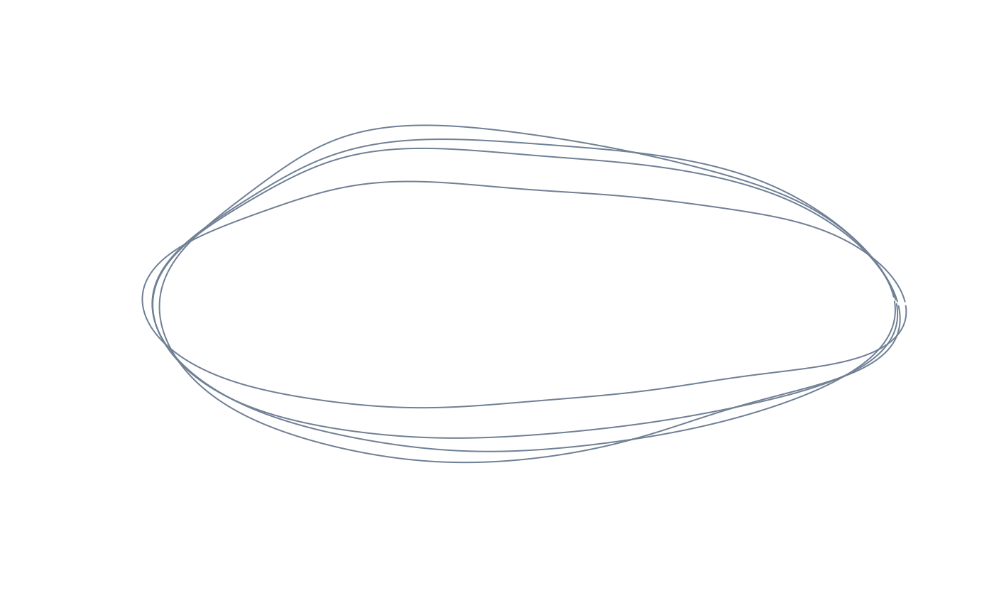
pile_shapes(sp_shapes, mshape = FALSE)


#mean shape of P. esbelta
esbelta_shape <- expected_shapes(shapes, x = shells$data$species,
                                 xvalue = "esbelta")
plot(inv_efourier(esbelta_shape, nb.pts = 200), type = "l")


#shapes expected by the linear regression of size on shape
exp_shapes <- expected_shapes(shapes, x = shells$sizes)
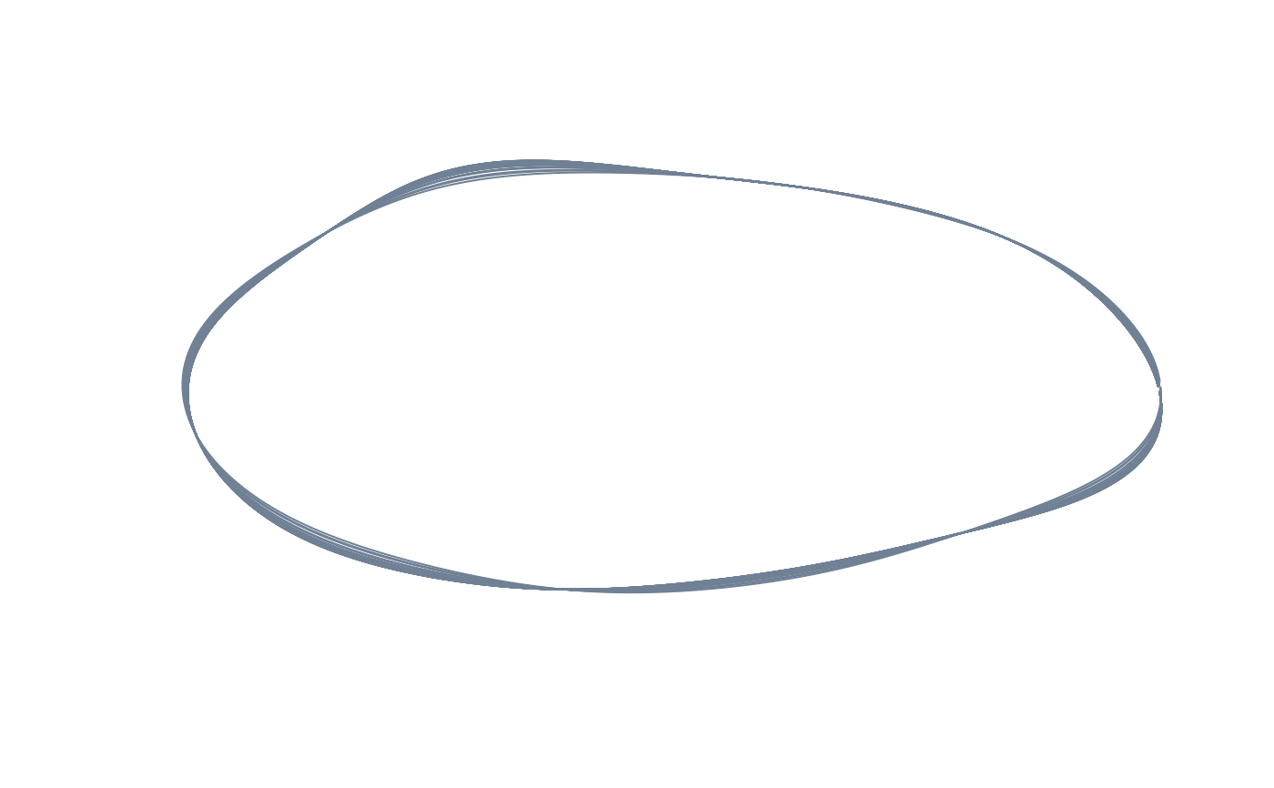
pile_shapes(exp_shapes, mshape = FALSE)


#shapes expected at the minimum size
large_shape <- expected_shapes(shapes, x = shells$sizes,
                               xvalue = min(shells$sizes))
plot(inv_efourier(large_shape, nb.pts = 200), type = "l")