Project landscape into morphospace

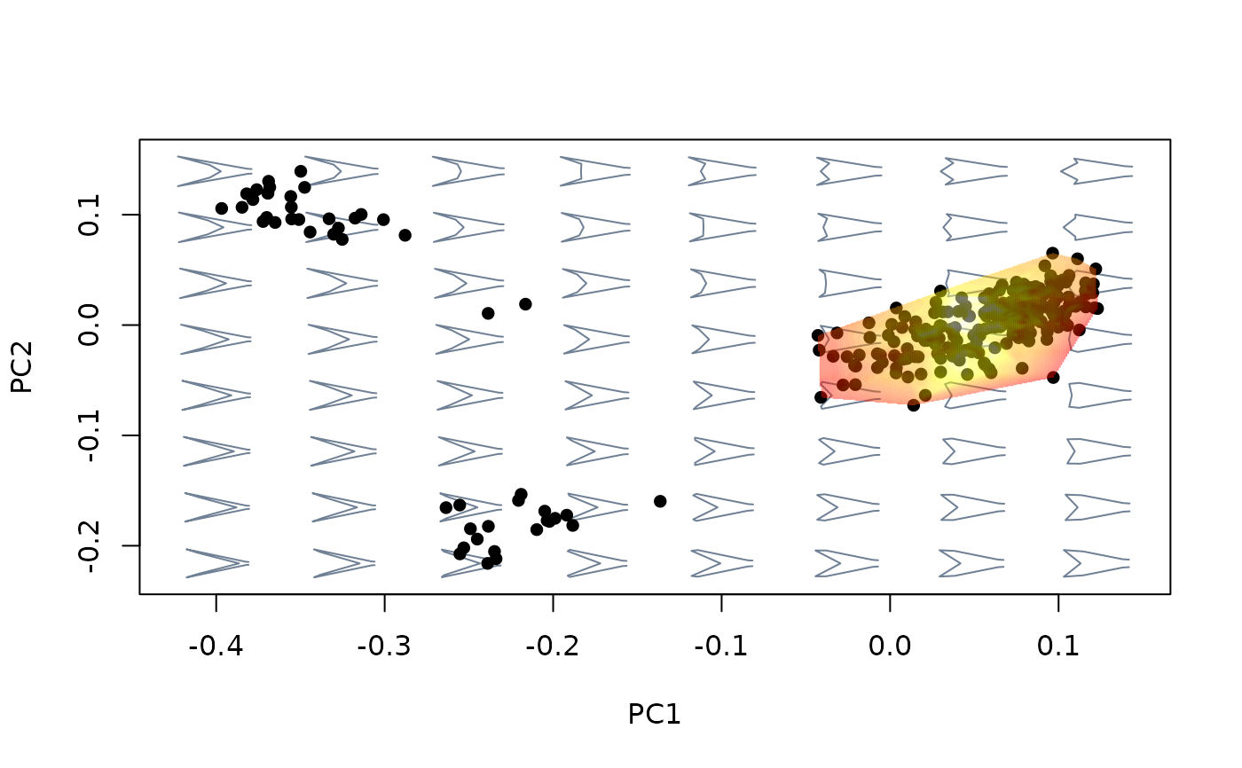
Compute and project a landscape surface as a contour map over an existing morphospace.

proj_landscape(
  mspace,
  shapes = NULL,
  FUN = NULL,
  X = NULL,
  linear = FALSE,
  resolution = 50,
  expand = 1,
  display = "contour",
  nlevels = 50,
  palette = grDevices::heat.colors,
  alpha = 0.5,
  lwd = 1,
  lty = 1,
  drawlabels = FALSE,
  spar = 0.5,
  pipe = TRUE,
  ...
)

Arguments

mspace

An "mspace" object.

shapes

Optional shape data. If provided, a landscape will be computed for the region of the morphospace encompassing that sample of shapes ("empirical landscape"). If NULL, the landscape will be computed for the set of background shape models ("theoretical landscape").

FUN

An optional ad hoc function to be applied to a set of shapes, stored in "two-dimensional" format, along its first margin (i.e. rows), and returning a single numeric value from each.

X

An optional vector containing the values assigned to each shape (vector length and order must match those from the shapes provided in shapes or from the background shape models, depending on whether or not shapes have been provided).

linear

Logical; whether to use linear interpolation (if FALSE, a cubic spline interpolation is used instead. See akima::interp().

resolution

Numeric; the resolution used for interpolation.

expand

Numeric; Magnification factor to extend (adjust) the reach of the landscape, attained by extrapolating the x, y, and z values. Only available for linear = FALSE.

display

Either "contour" or "filled.contour". For bivariate landscapes only.

nlevels

Number of levels (i.e., contours) to use for landscape representation.

palette

A function defining a color palette to use for landscape representation.

alpha

Numeric; transparency factor for filled contours.

lwd

Integer; width of the lines depicting contours.

lty

Integer; type of the lines depicting contours.

drawlabels

Logical; should the labels indicating the value of each surface contour be plotted?

spar

Numeric; smoothing parameter used to smooth landscape outline in univariate representations.

pipe

Logical; is the function being included in a pipe?

...

Further arguments passed to FUN.

Value

If a plot device with a morphospace is open, the landscape surface is projected into it as a contour map using akima::interp(). If pipe = FALSE, a list containing the x, y and z values used to plot the landscape (x and z for univariate morphospaces) is returned invisibly. If pipe = TRUE the supplied "mspace" object will be modified by appending a $landsc slot to $projected, as well as by adding some graphical parameters (stored into the $plotinfo slot), and returned invisibly.

Details

The purpose of this function is to generate and depict a 2- (for univariate morphospaces) or 3-dimensonal (for bivariate morphospaces) surface (i.e., a landscape), interpolated from values assigned to the set of shapes projected into an existing morphospace. These can be a sample of shapes specified by the user, producing a surface for a specific region of the morphospace ("empirical landscapes"). Alternatively, the set of background shape models can be used to generate a surface for the entire observed morphospace ("theoretical morphospace"). Generally, the values that are interpolated will represent a variable measuring functional performance (although it can be any kind of continuous variable), and can be either provided directly through the X argument or computed automatically using an ad hoc function through the FUN argument.

If the FUN argument is used, the function supplied must include a model argument feeding the ad hoc function with a single shape (stored as a vector of shape descriptors), and return a single numeric value computed for or from that shape. If the X argument is used instead, values should be in the same order than the shapes provided in shapes, or than the background shape models (i.e., from left to right and from bottom to top; see morphogrid, plot_morphogrid2d and plot_morphogrid3d) if shapes = NULL. Otherwise, landscape topography will be dissociated from the shapes represented in the morphospace. See examples below.

Directly providing the values to be interpolated using X can be useful when importing variables obtained using other software or pipelines. If the user desires to compute those variables for the background shape models, they can be extracted using extract_shapes) prior to exporting or feeding them to their preferred analytical protocol.

See also

morphogrid, mspace, plot_morphogrid2d, plot_morphogrid3d, extract_shapes

Examples

#load data and packages
library(geomorph)
library(Morpho)
library(Momocs)

data("tails")
shapes <- tails$shapes
links <- tails$links
type <- tails$data$type


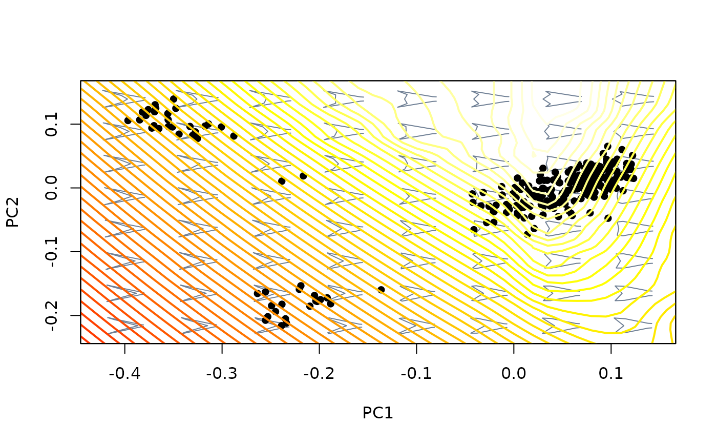
#Compute and plot adaptive landscape for wing tail shape:

##Using the FUN argument

###"Theoretical" landscapes

#plot morphospace with its associated adaptive landscape
mspace(shapes, links = links, nh = 8, nv = 8, size.model = 1.5,
       cex.ldm = 0) %>%
  proj_shapes(shapes, pch = 16) %>%
  proj_landscape(nlevels = 60, FUN = morphospace:::computeLD, expand = 1.2,
                 lwd = 2)


##Using the X argument

#first, create morphospace and extract background shapes without plotting
msp <- mspace(shapes, links = links, nh = 8, nv = 8, size.model = 1.5,
              cex.ldm = 0, plot = FALSE)
shapemodels2d <- two.d.array(extract_shapes(msp)$shapes)
#> Warning: there are no templates to warp; won't be returned

#run computeLD through the "two-dimensional" matrix of shapes models (this is
#the same thing the proj_landscape function is doing internally when FUN is
#used, but this vector could be replaced with some other variable obtained in
#a different way)
LDs <- apply(X = shapemodels2d, FUN = morphospace:::computeLD, MARGIN = 1)

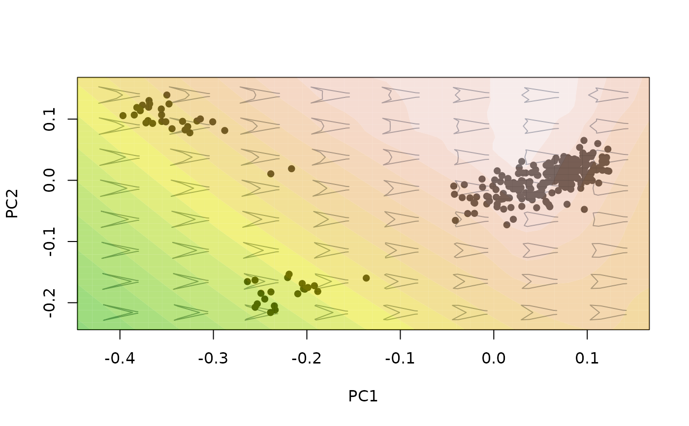
#second, plot morphospace with its associated adaptive landscape
msp <- mspace(shapes, links = links, nh = 8, nv = 8, size.model = 1.5,
              cex.ldm = 0) %>%
  proj_shapes(shapes, pch = 16) %>%
  proj_landscape(nlevels = 20, X = LDs, expand = 1.2,
                 palette = terrain.colors, display = "filled.contour")


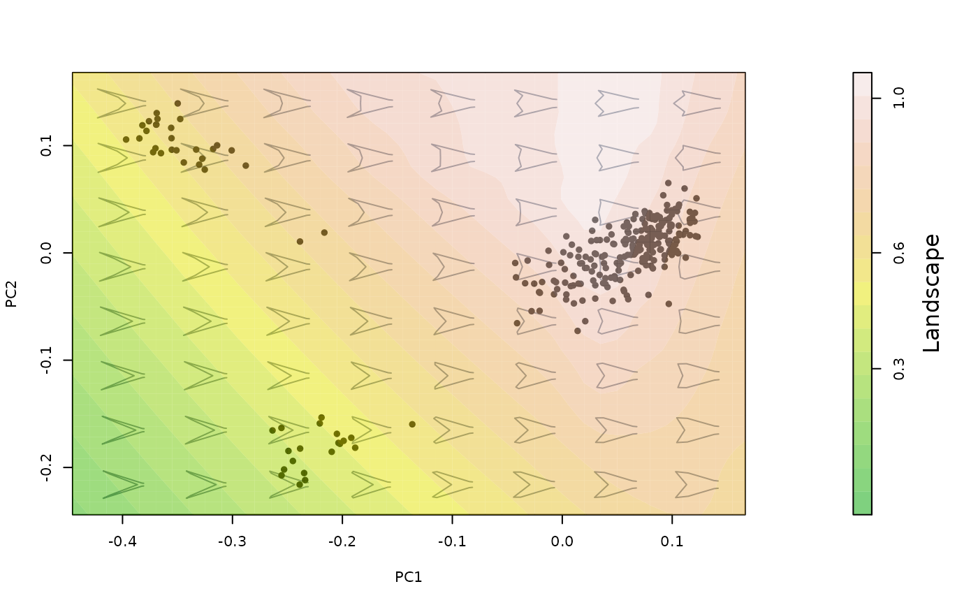
#add scalebar using plot_mspace()
plot_mspace(msp, scalebar = TRUE)


#be careful to use the same morphospaces in the second and first steps.
#For example, retaining the LD values computed above but changing the axes
#represented by mspace will result in the same surface wrongly being
#projected over a different morphospace!
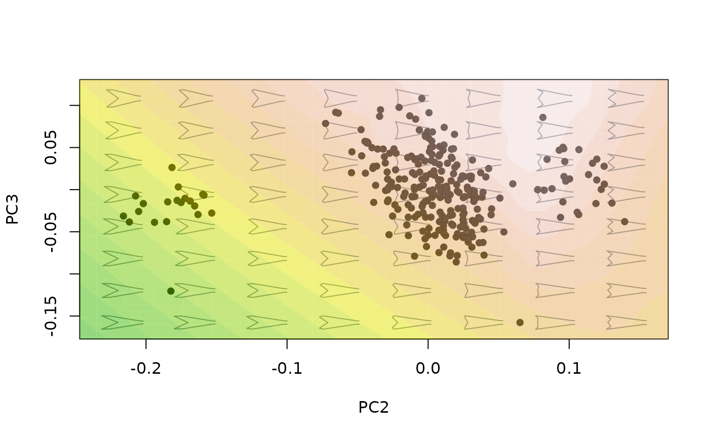
mspace(shapes, links = links, nh = 8, nv = 8, size.model = 1.5,
       cex.ldm = 0, axes = c(2,3)) %>%
  proj_shapes(shapes, pch = 16) %>%
  proj_landscape(nlevels = 20, X = LDs, expand = 1.2,
                 palette = terrain.colors, display = "filled.contour")


###"Empirical" landscapes

#it is essentially the same, but providing a set of shapes with the shapes
#argument of proj_landscape. Let's compute it it only for Tyrannus species with
#non-deep forked tail shapes:
mspace(shapes, links = links, nh = 8, nv = 8, size.model = 1.5,
       cex.ldm = 0) %>%
  proj_shapes(shapes, pch = 16) %>%
  proj_landscape(shapes = shapes[,,type == "NDF"], nlevels = 20,
                 linear = TRUE, FUN = morphospace:::computeLD, expand = 1.2,
                 display = "filled.contour")


#in this case, the resolution of the projected surface can be improved using
#the argument resolution (however, be aware this can be computationally
#intense! especially if a theoretical landscape is being computed)
mspace(shapes, links = links, nh = 8, nv = 8, size.model = 1.5,
       cex.ldm = 0) %>%
  proj_shapes(shapes, pch = 16) %>%
  proj_landscape(shapes = shapes[,,type == "NDF"], nlevels = 20,
                 linear = TRUE, resolution = 200,
                 FUN = morphospace:::computeLD, expand = 1.2,
                 display = "filled.contour")